Project 1: Images of the Russian Empire

Background

Sergei Mikhailovich Prokudin-Gorskii was a pioneering photographer who, in the early 20th century, undertook an ambitious project to document the Russian Empire in color. He captured thousands of scenes on glass plates using a unique technique: three separate exposures of the same subject, each filtered with red, green, and blue light. His vision was to use these images for educational purposes, but his plans were cut short by the Russian Revolution. Fortunately, his glass plate negatives survived and are now preserved by the Library of Congress, offering a vivid glimpse into a bygone era.

Project goals

The objective of this project is to take Prokudin-Gorskii's digitized glass plate negatives and digitally reconstruct the original color photographs. The core challenge involves image alignment. Each glass plate contains three distinct monochromatic images (red, green, and blue channels) that are slightly misaligned. The task is to use image processing techniques to automatically align these three channels, stacking them to form a single, correctly colored RGB image with minimal visual artifacts. This requires a robust and efficient alignment algorithm that can handle large, full-size images and produce a high-quality final result.

Part 1.1: Single-scale implementation for aligning small images

Process

A naive stack of BGR channels with no alignment

We start with a roll of film scan, with blue, green, and red channels list in order in the image. First, slice the image to get individual channels, each channel sharing the same width and height with the others.

A naive way to align them is to just stack all three channels together, with no alignment algorithm. This is not ideal, as we could see the edges of the object are not aligned.

To improve from the naive method, We could try "shifting" the images around and see how the result looks when we stack the channels onto each other. We could have a shift range of (-30, 30), and stack the BGR channels together two by two, then align both stacked images using the common image as a reference. To measure how good the alignment is, we could use some metrics here.

Metrics: The simplest metric we could use is just the L2 norm of the two images, also known as the Euclidean Distance which is simply

$\sqrt{\sum{\sum(image1(x,y)-image2(x,y))^2}}$

Another metric we could use is Normalized Cross-Correlation (NCC),

$NCC(A, B) = \frac{\sum_i(A_i - \overline{A})(B_i - \overline{B})}{\sqrt{\sum_i{(A_i - \overline{A})}^2{(B_i - \overline{B})}^2}}$

I used search range (-30, 30) with both the L2 and NCC metric, and both metrics yielded the same shift positions for all three small-scaled images, though L2 norm runtime is a lot faster than NCC due to runtime complexity.

Crop out borders: A trick I used is to get better alignment is to crop out the borders of the BGR channel images before alignment. This ensures that the alignment is less affected by lens imperfections and photo plat degredations. In this section, I cropped out a fixed value of 50 pixels each on the left, right, top, and bottom side of the BGR images before aligning them.

Scroll to see alignment results:

CATHEDRAL.jpg

Best shift for G: (-7, -1)

Best shift for B: (-12, -3)

Runtime using L2: 0.5654s

Runtime using NCC: 2.2401s

MONASTERY.jpg

Best shift for G: (-6, -1)

Best shift for B: (-3, -2)

Runtime using L2: 0.5802s

Runtime using NCC: 2.0185s

TOBOLSK.jpg

Best shift for G: (-4, -1)

Best shift for B: (-6, -3)

Runtime using L2: 0.5654s

Runtime using NCC: 2.3110s

Part 1.2: Multi-scale alignment of large images

Metric selection

The images to be matched do not necessarily have the same brightness values (they are different color channels).

Problem with L2 norm: Because the L2 norm involves squaring pixel values, very bright pixels of high intensity would contribute significantly more to the total sum than do dark pixels of low intensity. This causes the overall metric to be heavily influenced by bright areas, making it "sensitive" to highlights and bright spots. Because the images to be matched do not actually have the same brightness values (they are different color channels), we would need a better metric for alignment.

NCC is robust to linear changes in brightness, because when we subtract the mean intensity from each pixel, we are eliminating the effect of any constant brightness offset. We get the normalized cross-correlation by dividing by the standard deviation. This normalization scales each pixel to have "unit variance," canceling out any constant multiplicative contrast changes. 

Dealing with larger images: Image Pyramids

Surely we could increase the search range from Part 1.1 as the image size increases, but this would become prohibitively expensive when the image becomes too large. In this case, we would need a faster search procedure to help us summarize and abstract information from the large-scale image.

An image pyramid could be very helpful in this case. An image pyramid represents the image at multiple scales (usually scaled by a factor of 2) and the processing is done sequentially starting from the coarsest scale (smallest image) and going down the pyramid, updating your estimate as you go. In this section, I created an image pyramid with 4 levels, image at each level being half the width and height of its previous level.

Given the initial position (a, b), and a shift position (x, y) for the coarsest image, we can then search in the next level of the image pyramid at position (2x + a, 2y + b), with search range = (-1, 1) to compensate for any rounding lost in the rescale (division) of 2. Using this, we can keep updating our NCC score and go all the way up to the largest-scaled image in the pyramid, to get the best shift with the highest NCC score possible.

Crop out borders aggressively: I cropped out a fixed value of 200 pixels each on the left, right, top, and bottom side of the BGR images before aligning them. Since lens imperfections and photo plat degredations get worse as pixels are far from the center, cropping pixels out and leaving important details in the center for alignment ensure that the alignment is more accurate and less affected by the quality of the film scan.

Compute NCC score using overlapping pixels only

One trick I used to improve accuracy in alignment was to ensure that I'm only computing the NCC score in the strictly overlapping window of the two images. For example, given two images A and B of size (w, h), if the alignment requires shifting image B to the right with value x (x > 0) and to the bottom with value y (y > 0), then I only compute NCC score using

$B[x:, y:]$

This is a side-by-side comparison of the Image Pyramid + NCC score method, computed with all pixels in images vs. only using overlapping pixels. We could see that the naive computation has the blue channel misaligned quite far to the right side, while the NCC score using overlapping pixels gives us higher NCC score (an dhigher correlation), and better alignment result.

Scroll to see alignment results:

Here are the fixed parameters I used for the alignment alogrithm:

EMIR.jpg

Best shift for G: (-57, -17)

Best shift for B: (-74, -44)

Runtime: 10.1009s

ITALIL.jpg

Best shift for G: (-38, -15)

Best shift for B: (-76, -35)

Runtime: 9.7821s

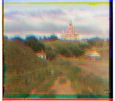
CHURCH.jpg

Best shift for G: (-33, 8)

Best shift for B: (-58, 5)

Runtime: 9.3598s

THREE_GENERATIONS.jpg

Best shift for G: (-58, 2)

Best shift for B: (-111, -10)

Runtime: 9.6963s

LUGANO.jpg

Best shift for G: (-52, 12)

Best shift for B: (-92, 28)

Runtime: 9.9049s

MELONS.jpg

Best shift for G: (-96, -3)

Best shift for B: (-178, -12)

Runtime: 9.6809s

LASTOCHIKINO.jpg

Best shift for G: (-78, 7)

Best shift for B: (-75, 9)

Runtime: 10.0418s

ICON.jpg

Best shift for G: (-48, -5)

Best shift for B: (-89, -23)

Runtime: 10.4537s

SIREN.jpg

Best shift for G: (-47, 18)

Best shift for B: (-95, 25)

Runtime: 10.5801s

SELF_PORTRAIT.jpg

Best shift for G: (-98, -8)

Best shift for B: (-176, -36)

Runtime: 10.0840s

HARVESTERS.jpg

Best shift for G: (-65, 3)

Best shift for B: (-124, -13)

Runtime: 9.6655s

Scroll to see more examples from the Prokudin‑Gorskii collection

CASTLE.jpg

Best shift for G: (-46, 9)

Best shift for B: (-79, 25)

Runtime: 10.6426s

DOME.jpg

Best shift for G: (-54, 2)

Best shift for B: (-96, -5)

Runtime: 9.5361s

MOSQUE.jpg

Best shift for G: (-44, -1)

Best shift for B: (-70, -11)

Runtime: 9.5197s

KHIVA.jpg

Best shift for G: (-53, 17)

Best shift for B: (-94, 7)

Runtime: 10.1706s

Zoomed-in view of the minor misalignment

Issue with the NCC + Image Pyramid method: NCC + Image Pyramid method overall yields accurate result for all images, with an exception of a minor glitch in the EMIR.tif image alignment. If we zoom into the EMIR.tif alignment result, we could see a yellow cast on Emir's head, possibly due to misalignment of the blue channel.

Part 2.1: Better alignment: Multi-scale alignment using NCC and Laplacian Pyramids

The NCC + Gaussian image pyramids method in Part 1.2 wasn't ideal. Despite 13 out of 14 images in the data file aligned pretty accurately, the EMIR.tif failed to be algined perfectly. The red and green channels were aligned perfectly, but the blue channel of EMIR.tif was slightly below the two, creating a yellow cast that's quite obvious on Emir's head and facial features.

Illustration of Laplacian Pyramid

To fix this, I wondered if better features could be used for the alignment, instead of simply the raw RGB pixels. One intuitive enhancement from the current approach is to use Laplacian Pyramids, instead of the current Gaussian Pyramids in Part 1.2.

Laplacian pyramids are constructed from Gaussian pyramids by subtracting the next level’s upsampled Gaussian image from the current level’s Gaussian image.$$L_i = G_i - \operatorname{expand}(G_{i + 1})$$This subtraction removes low-frequency content (i.e., smooth/blurred areas), and preserves the high-frequency details that are lost in the Gaussian blur, such as edges and fine textures. As a result, Laplacian pyramid levels contain mostly zero or near-zero values in flat regions, and non-zero edge-like traces where there are intensity transitions. This makes the Laplacian pyramid ideal for tasks that benefit from highlighting structural information, such as image alignment, blending, and compression.

Constructing the Laplacian Pyramid

Below is the Laplacian Pyramid of 4 levels created for EMIR.tif . Each level is 1/4 of the previous level's size, and the edges are more and more obvious as we go up in the pyramid. The level 4 image has thicker "strokes," which summarized key edges in EMIR.tif after several layers of gaussian blurring.

LEVEL 0

Image size: (3208, 3702)

LEVEL 1

Image size: (1604, 1851)

LEVEL 2

Image size: (802, 926)

LEVEL 3

Image size: (400, 463)

Using the Laplacian Pyramid generated above, and the NCC metric from Part 1.2, the alignment is a lot more accurate now.

EMIR_LAPLACIAN.jpg

Method: NCC + Laplacian Pyramids

Best shift for G: (-57, -17)

Best shift for B: (-105, -41)

Runtime: 9.8312s

Here is a zoomed-in comparison of the two methods. Just looking at Emir's head, the yellow cast due to blue channel's misalignment disappeared after aligning the source image with the Laplacian Pyramid above. All other images were aligned accurately with this method as well.

EMIR.jpg

Best shift for G: (-57, -17)

Best shift for B: (-105, -41)

Runtime: 9.8079s

ITALIL.jpg

Best shift for G: (-38, -14)

Best shift for B: (-77, -36)

Runtime: 10.7475s

CHURCH.jpg

Best shift for G: (-33, 8)

Best shift for B: (-58, 4)

Runtime: 10.1170s

THREE_GENERATIONS.jpg

Best shift for G: (-57, 5)

Best shift for B: (-114, -11)

Runtime: 10.0456s

LUGANO.jpg

Best shift for G: (-54, 14)

Best shift for B: (-92, 29)

Runtime: 10.9043s

MELONS.jpg

Best shift for G: (-96, -4)

Best shift for B: (-178, -14)

Runtime: 10.9904s

LASTOCHIKINO.jpg

Best shift for G: (-77, 7)

Best shift for B: (-75, 8)

Runtime: 10.9783s

ICON.jpg

Best shift for G: (-48, -5)

Best shift for B: (-89, -23)

Runtime: 11.2596s

SIREN.jpg

Best shift for G: (-47, 19)

Best shift for B: (-97, 24)

Runtime: 11.6070s

SELF_PORTRAIT.jpg

Best shift for G: (-98, -8)

Best shift for B: (-181, -37)

Runtime: 11.5348s

HARVESTERS.jpg

Best shift for G: (-65, 3)

Best shift for B: (-124, -12)

Runtime: 10.8357s

Part 2.2: Automatic cropping

1. Preprocess with cropping: I first crops the central 60% of the image. This eliminates irrelevant outer edges, ensuring the algorithm focuses only on the primary content.

2. Detect edges: Then we use the Canny edge detection algorithm on each color channel (red, green, blue) of the central crop, to find sharp changes in pixel intensity. These changes represent the image's boundaries.

3. Identify lines: In order to find the straight lines (film scan borders to remove), I use the Hough Transform. It efficiently identifies the lines that form the border of the photograph or subject matter.

4. Then I define the bounding region of the image and find the minimum and maximum x and y coordinates.

5. Final crop: The coordinates are then scaled back to the original image's dimensions. I added a 1% buffer margin is added to prevent cutting into the main subject. The image is then cropped to this final, refined bounding box, and the result is saved.

EMIR.jpg

ITALIL.jpg

CHURCH.jpg

THREE_GENERATIONS.jpg

LUGANO.jpg

MELONS.jpg

LASTOCHIKINO.jpg

ICON.jpg

SIREN.jpg

SELF_PORTRAIT.jpg

HARVESTERS.jpg

Part 2.3: Automatic contrast

Linear contrast stretching

One intuitive way to adjust contrast is just to stretch the pixel intensity range of an image so that the minimum pixel value becomes 0 and the maximum becomes 1. This allows to effectively maximize the image’s contrast in a linear way. This is called linear contrast stretching.

Let the minimum pixel intensity across the entire image be a, and the maximum pixel intensity across the entire image be b. In order to perform linear transformation, each pixel value x is transformed using the formula:$$x’ = \frac{x - a}{b - a}$$

This transformation ensures: when x = a, then x’ = 0; when x = b, then x’ = 1; all other values x are linearly mapped into the interval [0, 1].

Below is the before and after of the linear stretch, and visually the two images look identical.

Original contrast

Linear contrast

The two images above look identical. Why is that?

The problem with linear contrast stretching is that for an float32 image that has pixel min value = 0 and max value = 1, the pixel intensity band would not be stretched at all, as the range before and after the stretch would be the same. This would result in the post-processed image looking exactly the same as the image without adjusting contrast.

Histogram Equilization

To address this issue, we could use histogram equilization to redistribute the pixel intensity. Histogram equilization transforms the original pixel intensity histogram into a new histogram that is more uniform and covers a wider intensity range. I used the histogram equilization function from skimage.exposure package.

Original contrast

Histogram Equilization

To verify that automatic contrast works, below is a comparison of the two contrast adjusting methods, with respect to the original image aligned with NCC + Laplacian pyramid. As one can tell, the contrast in the histogram-equilized image is very sharp.

EMIR.jpg

ITALIL.jpg

CHURCH.jpg

THREE_GENERATIONS.jpg

LUGANO.jpg

MELONS.jpg

LASTOCHIKINO.jpg

ICON.jpg

SIREN.jpg

SELF_PORTRAIT.jpg

HARVESTERS.jpg

Part 2.4: Automatic white balance

Automatic white balance involves two problems: estimating the illuminant, and manipulating the colors to counteract the illuminant and simulate a neutral illuminant. For estimating the illuminat, some simple methods including assuming the brightest color is the illuminant and shift those to value = 255 (white), or assuming the average color in the image is achromatic(gray) and adjust the average values of each channel to be equal. The former one is the White Patch algorithm, and the latter is called the Gray World algorithm.

I tried implementing both algorithms, but shifting the brighest pixel value to be 255 didn't yield any meaningful effect on EMIR.tif, because the brightest values of all three channels in EMIR.tif is (255, 251, 254). With the highest intensity value being so close to white, the white patch algorithm wouldn't be helpful in this case.

Therefore, I used the Gray World algorithm. I first get the mean of each BGR channels, then get the average mean of all channels M as the gray value of the image. Then I scaled the BGR channels linearly so that the average of each channel would be M. I also made sure to clip each channel's range at [0, 255] to avoid overflowing. Then, we have our white-balanced image using the Gray World algorithm. See below for the side-by-side before and after comparison.

Before and after of automatic white balance using the Gray World algorithm

Part 2.5: Better color mapping

When we have raw images from separate channels (like photographic plates with red, green, blue filters in this case), the channel responses do not necessarily match standard RGB. For example, the “red” channel might capture some green/blue light. Directly assigning these channels to RGB usually produces unrealistic colors. So, we need a mapping from raw channels to true RGB.

In order to make the photo more realistic, I wondered if we could customize a palette and adjust the pixels in the original image to be as close to the customered RGB palette as possible. I was inspired by the technique of using Van Gogh painting to adjust image colors.

IMG 2.5.1: Van Gogh sunflowers painting

Here, I used a VanGogh painting to create a cusotmized color palette, and mapped it to the Emir image using two different methods.

Method 1: k-means clustering From Van Gogh's paiting, I used k-means clustering to extract 8 dominant colors to compose the customized color palette.

Then, to apply the colors from the palette to the target image, I mapped image colors to the cloest colors in the palette, using k-d trees for efficient nearest-neighbor searches.

The mapped image 2.5.3 seems to have very "flat" colors(kind of posterized). This is due to the way we mapped the pixels. By using nearest neighbor mapping, every pixel in your photo is replaced by the single closest palette color from the cutomized palette. This means that the entire image is restricted to only N colors (e.g. I set N=8) with no gradients. This gives the “flat” look we're seeing.

Method 2: Floyd-Steinberg dithering To fix this and improve the visual asesthetic of the color mapped image, we could use Floyd–Steinberg dithering technique so that pixels “mix” palette colors instead of being flat. Floyd–Steinberg dithering reduces the number of colors in an image by distributing the quantization error of each pixel to its neighboring pixels, and convert images with high color depth to lower color palettes. Now we have a Van Gogh-style photo of Emir using color mapping.

IMG 2.5.2: Emir (original)

IMG 2.5.3: Emir (k-menas clustering)

IMG 2.5.4: Emir (Floyd-Steinberg dithering)

Making the photo more realistic: Similarly, we can create a customized RGB palette and apply Floyd-Steinberg dithering to make the photo look more realistic. Image 2.5.6 is the result, using a reference palette of only R, G, and B colors.

IMG 2.5.5: RGB reference image for palette

IMG 2.5.2: Emir (original)

IMG 2.5.6: Emir (RGB palette, Floyd-Steinberg dithering)