Part A.1: Shoot the Pictures

Below are three sets of images with projective transformations between them, with fixed center of projection. Part A of this project will use the three sets of images below to compose image mosaics using image warping and auto-stitching.

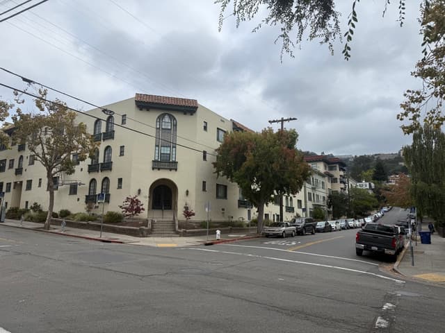
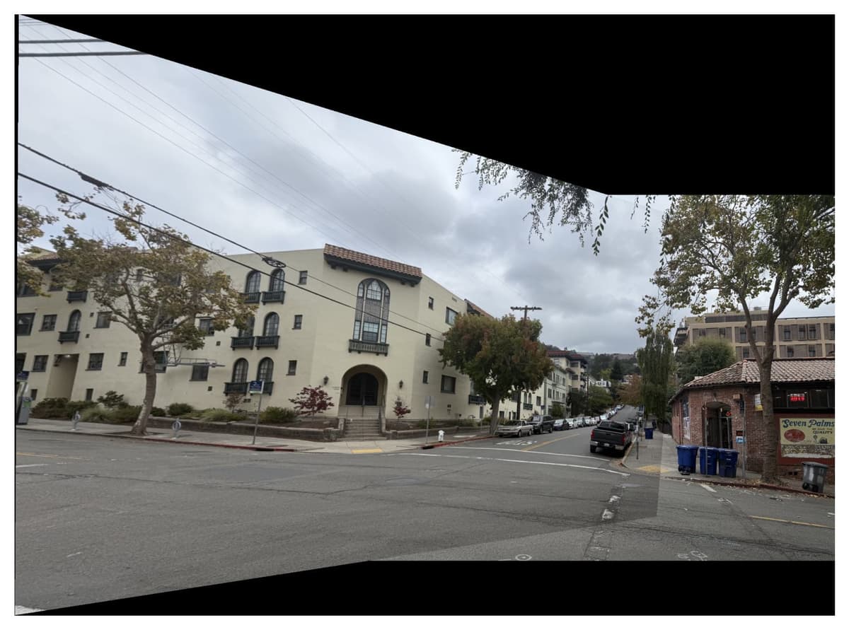
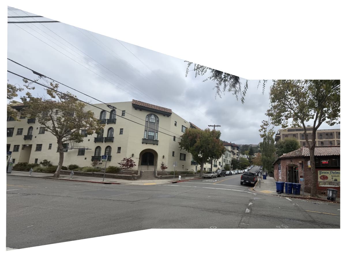
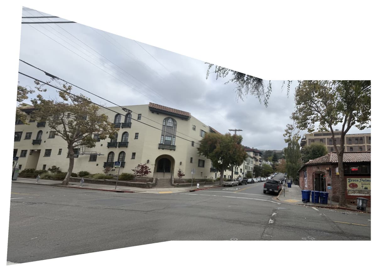
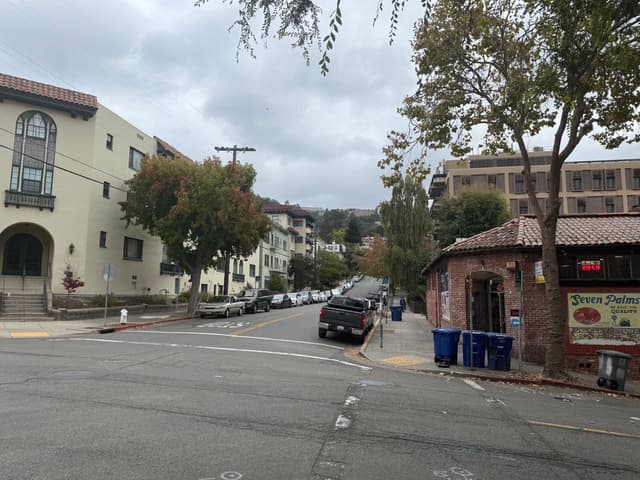
Street (left)

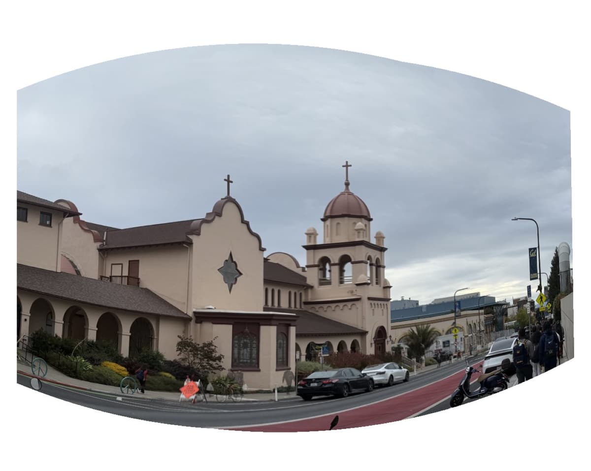
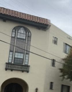
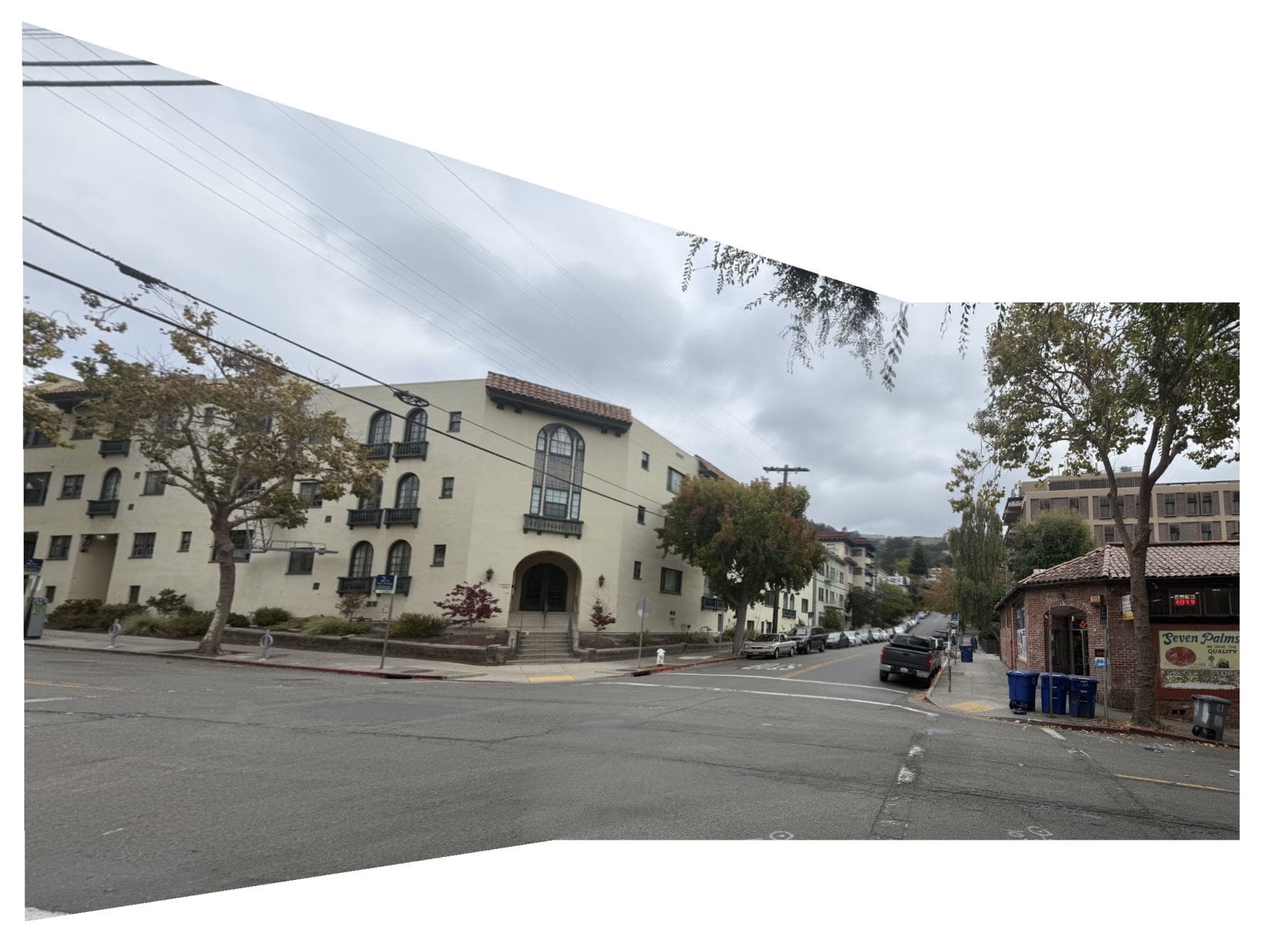
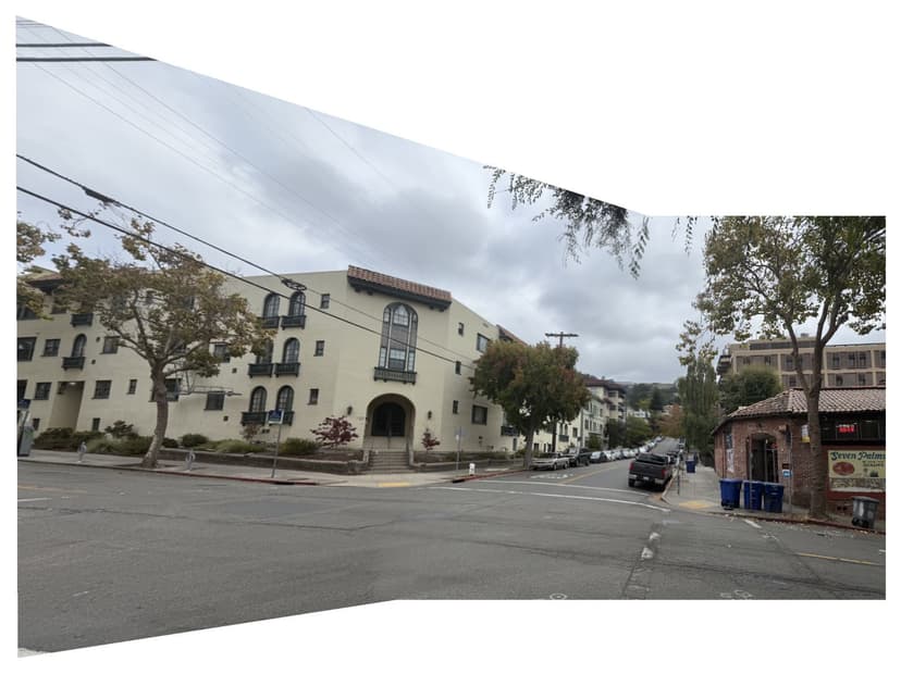
Campus (left)

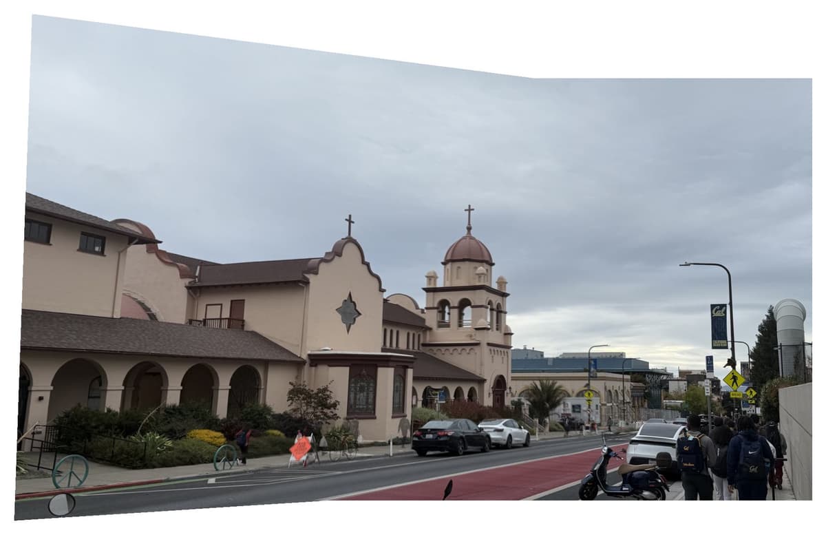
Campus (right)

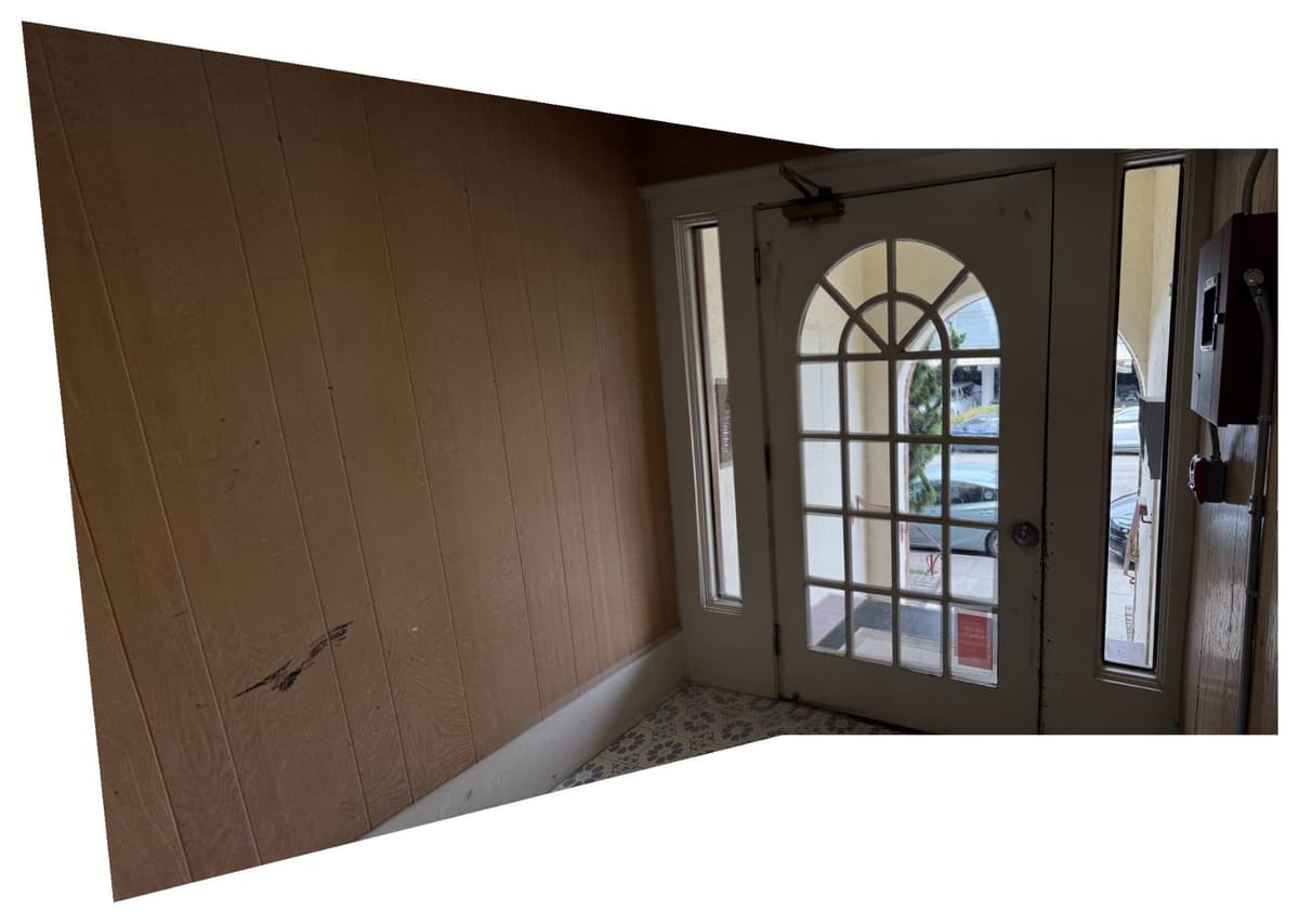
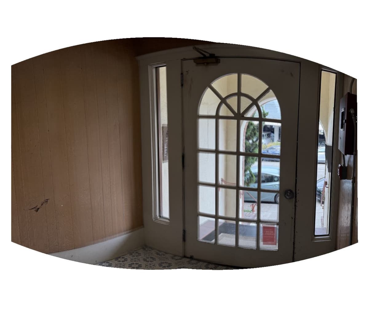
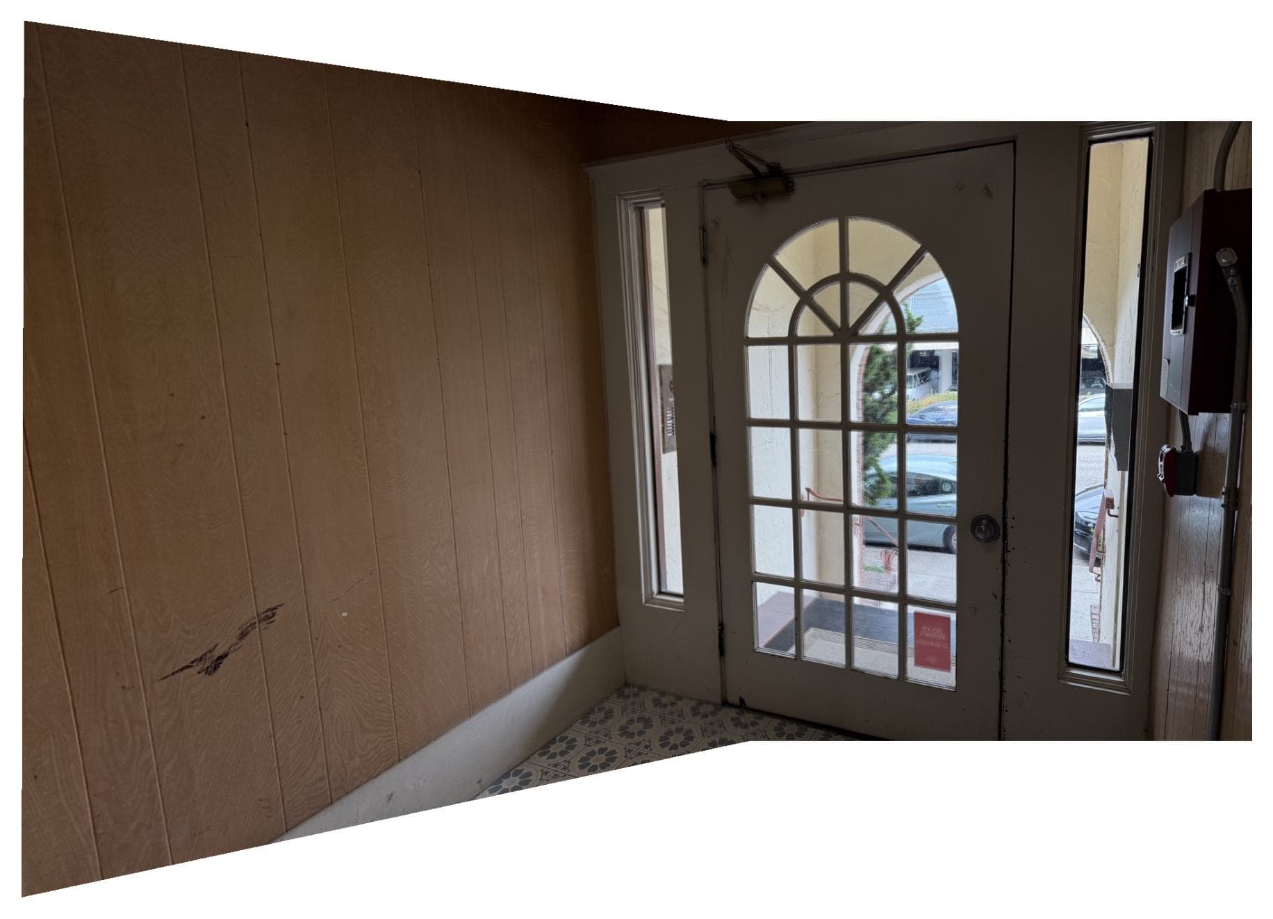
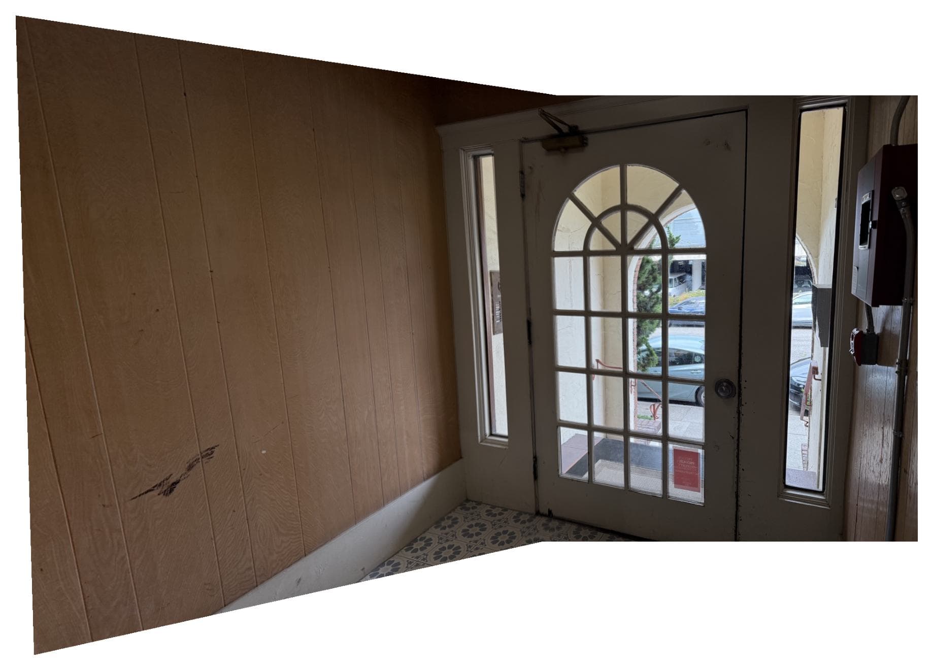
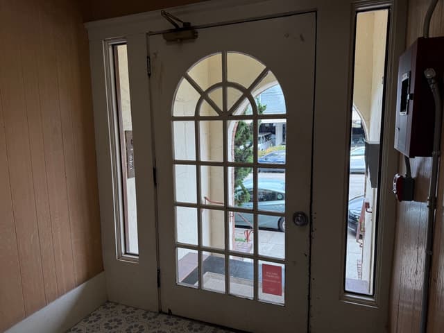
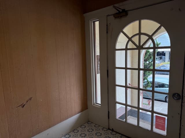
Door (left)

Part A.2: Recover Homographies

We know that for a pair of corresponding points $p = (x, y)^T$ and $p = (x^{prime}, y^{prime})^T$ ,

H = \begin{bmatrix} h_{11} & h_{12} & h_{13} \\ h_{21} & h_{22} & h_{23} \\ h_{31} & h_{32} & h_{33} \\ \end{bmatrix}

Since the homography is up to scale, we can set the 9th entry $h_{33} = 1$ . And therefore, we have eight unknowns

h = [h_{11}, h_{12}, h_{13}, h_{21}, h_{22}, h_{23}, h_{31}, h_{32}]^T

Given $p^{\prime} = Hp$ , we have

\begin{aligned} x' &= \frac{h_{11}x + h_{12}y + h_{13}}{h_{31}x + h_{32}y + 1} \\ y' &= \frac{h_{21}x + h_{22}y + h_{23}}{h_{31}x + h_{32}y + 1} \end{aligned}

Multiply both sides by the denominator, and rearrange both equations, we get the linear equations:

\begin{aligned} x h_{11} + y h_{12} + 1 h_{13} - x^{\\prime} x h_{31} - x^{\prime} y h_{32} &= x^{\prime} \\ x h_{21} + y h_{22} + 1 h_{23} - y^{\\prime} x h_{31} - y^{\prime} y h_{32} &= y^{\prime} \end{aligned}

In matrix form, we have $Ah = b$ , where

A = \begin{bmatrix} x & y & 1 & 0 & 0 & 0 & -x^{\prime}x & -x^{\prime}y \\ 0 & 0 & 0 & x & y & 1 & -y^{\prime}x & -y^{\prime}y \\ \end{bmatrix} ,\quad b = \begin{bmatrix} x^{\prime} \\ y^{\prime} \\ \end{bmatrix}

So for n pairs of corresponding points, A will be 2n x 8, and b will be 2n x 1.

A = \begin{bmatrix} x_{1} & y_{1} & 1 & 0 & 0 & 0 & -x_{1}^{\prime}x_{1} & -x_{1}^{\prime}y_{1} \\ 0 & 0 & 0 & x_{1} & y_{1} & 1 & -y_{1}^{\prime}x_{1} & -y_{1}^{\prime}y_{1} \\ x_{2} & y_{2} & 1 & 0 & 0 & 0 & -x_{2}^{\prime}x_{2} & -x_{2}^{\prime}y_{2} \\ 0 & 0 & 0 & x_{2} & y_{2} & 1 & -y_{2}^{\prime}x_{2} & -y_{2}^{\prime}y_{2} \\ \vdots & & & & & & & \vdots \\ x_{n} & y_{n} & 1 & 0 & 0 & 0 & -x_{n}^{\prime}x_{n} & -x_{n}^{\prime}y_{n} \\ 0 & 0 & 0 & x_{n} & y_{n} & 1 & -y_{n}^{\prime}x_{n} & -y_{n}^{\prime}y_{n} \end{bmatrix} ,\quad b = \begin{bmatrix} x_{1}^{\prime} \\ y_{1}^{\prime} \\ x_{2}^{\prime} \\ y_{2}^{\prime} \\ \vdots \\ x_{n}^{\prime} \\ y_{n}^{\prime} \end{bmatrix}

Identify correspondences: I picked roughly 20 points for each image set, for the best alignment effect. Below are the images set with corresponding points visualized.

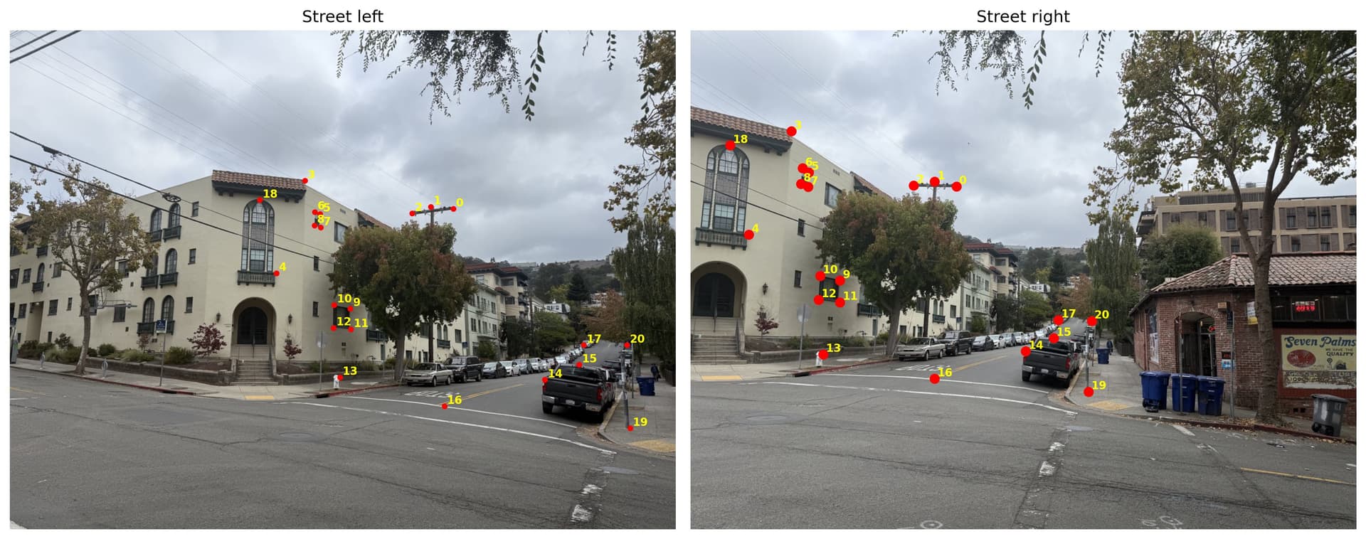
Street

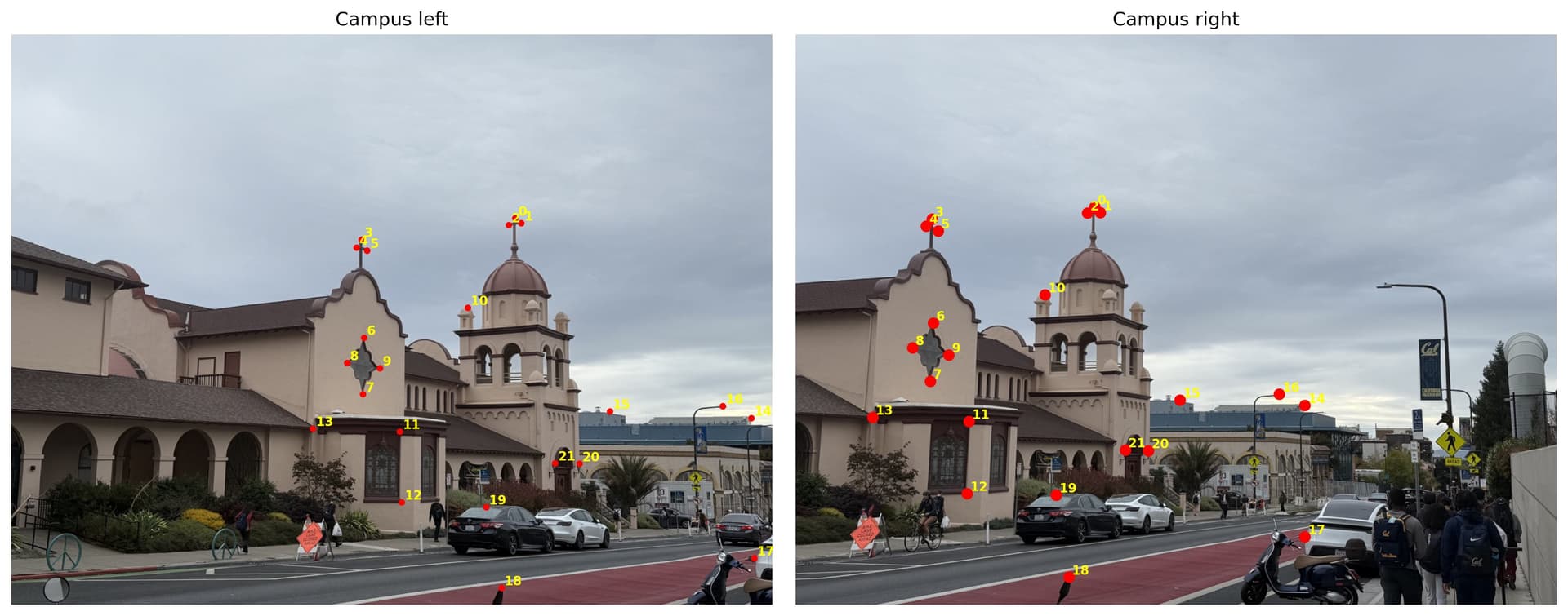
Campus

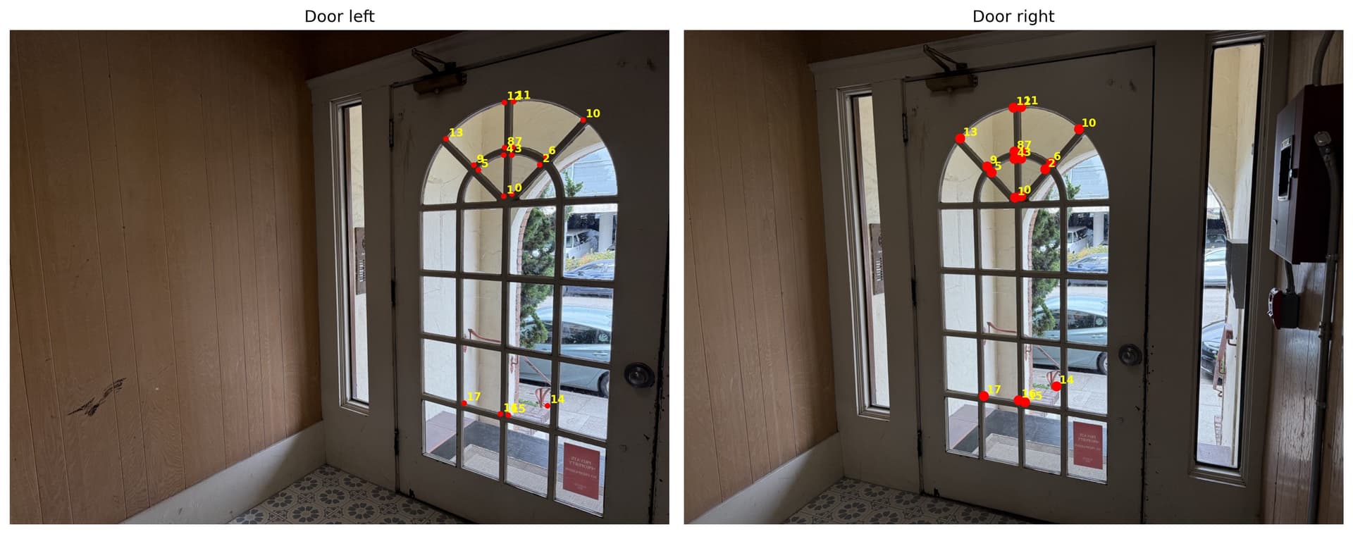
Door

Using the correspondences in street image set as an example, we have:

A = [[    852     343       1       0       0       0 -435372 -175273]
 [      0       0       0     852     343       1 -255600 -102900]
       ...     ...       ...   ...     ...   ...   ...   ...  
                      # omit equations for length
 [   1186     605       1       0       0       0 -914406 -466455]
 [      0       0       0    1186     605       1 -662974 -338195]]

 b = [511 300 469 291 429 298 194 194 112 393 227 273 215 265 226 301 212 295
 287 481 249 472 287 523 246 518 255 623 644 617 698 592 469 670 707 557
  76 221 765 695 771 559]

Compute H: To solve for h, we can use the least-squres where $h = (A^T A)^{-1} A^T b$ In code, I used

h, _, _, _ = np.linalg.lstsq(A, b, rcond=None)

to solve for the 8 unknowns, and append h_33 = 1 to the bottom right corner of the 3x3 matrix to get H. Below are the H matrices for each of the image sets above, using H = computeH(im1_pts,im2_pts):

street_H = [[ 2.06547633e+00 -7.53752292e-02 -8.61105758e+02]
 [ 4.64225435e-01  1.72607077e+00 -4.74795776e+02]
 [ 8.07725442e-04  7.38934331e-05  1.00000000e+00]]

campus_H = [[ 1.30642452e+00 -3.90497699e-02 -4.92878241e+02]
 [ 1.47561264e-01  1.19275602e+00 -1.45325762e+02]
 [ 2.38517397e-04 -6.17060967e-06  1.00000000e+00]]

door_H = [[ 1.89016788e+00  1.00929387e-01 -7.74849407e+02]
 [ 2.39590678e-01  1.61325228e+00 -2.08538936e+02]
 [ 6.62580476e-04  8.98712430e-05  1.00000000e+00]]

Part A.3: Warp the Images

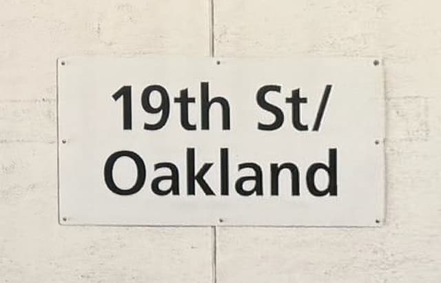
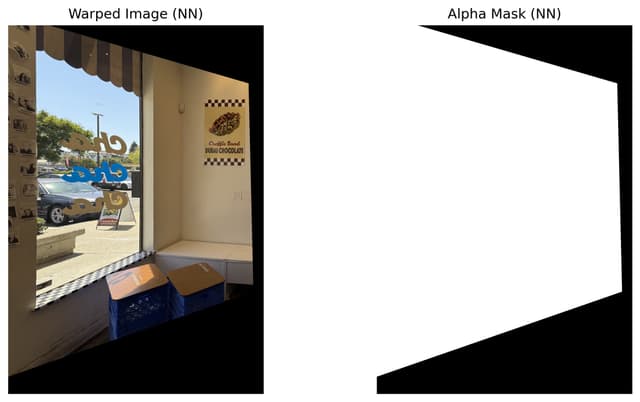
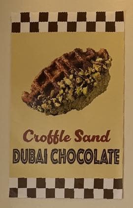
To ensure that all of the my code is correctly warping the images, I used two images with rectangular objects to test the warping algorithms. Below are two images, one taken in the 19th & Oakland Bart station, another taken in a coffee shop, and I used the Bart station sign and the coffee shop poster to retify the iamges. After setting the correspondences at each corner of the rectangular objects (Bart sign and coffee poster, respectively), I obtain the H value for each image. This H value would warp the input objects that are skewed in the input image back to rectangular shapes via projective transformation.

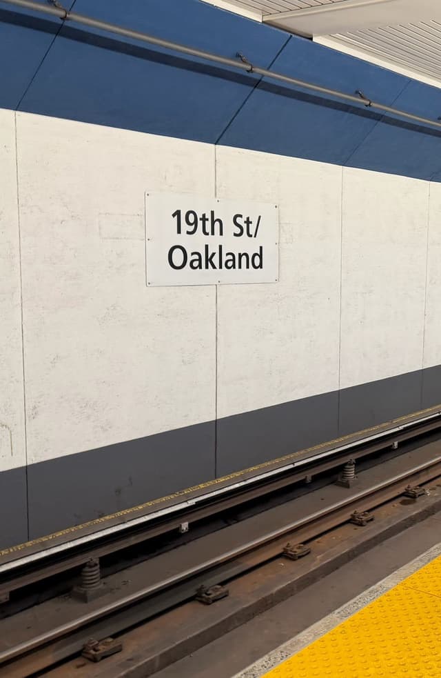
Bart

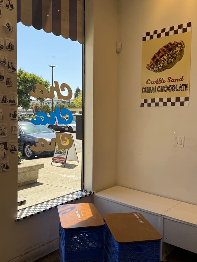
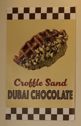
Cafe

Compare interpolation methods: I applied inverse warping to avoid holes in the output image, and used two methods for the warping algorithms. Here is a comparison between neartest-neighbor and bilinear warping using the Bart image. We can see that nearest neighbor is the faster, since it just finds the nearest pixel in the source image and use its intensity. Bilinear is slower, as it requires computing the new pixel intensity using weighted average of the four nearest pixels around it.

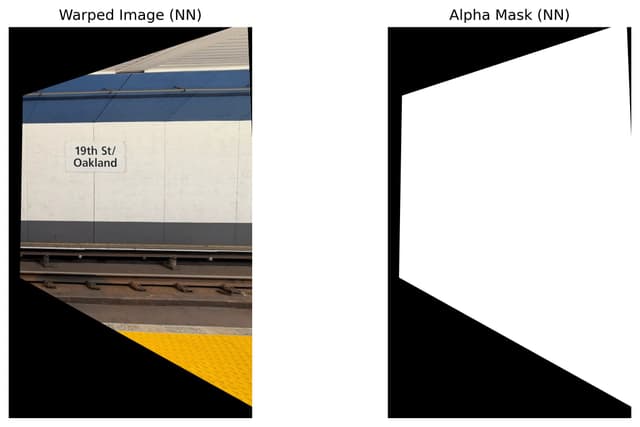
Bart rectified (nn)

1.8761 seconds

Bart rectified (bilinear)

3.9961 seconds

Bart rectified detail (nn)

Bart rectified detail (bilinear)

I also notice that the image warped with bilinear interpolation has finer details. This is especially obvious in the cafe detail comparison below. This is because nearest neighbor only copies the pixel value from the source image in the warped image; with inverse warping, some areas would have the same pixel value, producing a lower-resolution visual effect. But with bilinear interpolation, the warped image would have a smoother transition from areas corresponding to one source pixel to another.

Cafe rectified (nn)

0.2243 seconds

Cafe rectified (bilinear)

0.3706 seconds

Cafe rectified detail (nn)

Cafe rectified detail (bilinear)

Part A.4: Blend the Images into a Mosaic

1. Building a new canvas

Warp image to find new corners: First, I transform the source image using the H matrix we have computed from Part A.2. It is worth noticing that Ah = b warps source image 1 to be in the frame of source image 2, so the first step here is to warp all four corners of the image 1 (aka the left images in all image sets) to the frame of image 2 (the right images).

Compute new image frame: Now the two images are both in the right image's frame, we can compute the corners of the combined image. I get the min and max values of (x, y) by looking at four corners of the warped left image and the 4 corners of the right image. Since we cannot guarantee the warped image would be right at the top left corner of the mosaic image, I apply a translation matrix to shift the combined image to remove paddings and ensure all parts of the new image is in frame.

Warp left image and apply to canvas:Now that we have computed the size of the combined image, what we have essentially is an empty canvas for us to apply the source images onto. To start, I warp the left image using bilinear interpolation and add any paddings on the horizontal or vertical edges if needed, to ensure that the warped left image is the same size as the canvas. This ensures that all pixels in the warped left image directly corresponds to the pixels on canvas. Then I write the warped image to the canvas.

2. Blending two images together

Naive approach: directly overwrite the canvas with the second imageA naive approach here is to apply the right image to the canvas, and overwrite the overlapping area. See below for the effect. We can see that this method is not ideal, as the edges of the left image is very obvious. To remove this edge effect, could we use some average of the two images to better blend them together?

Street mosaic, overwrite

Second approach: taking the average of the two images in the overlapping areaI then built a mask for the overlapping area of the two images, and took half of the pixel intensity in the left image and half of the pixel intensity in the right image within the overlapping area. The equation to compute the canvas image is:

I = 0.5 I_1 + 0.5 I_2

This was an attempt to blend the two images together, but the visual seams are still very obvious. Using this method, we still have full weight for one image on one side, and full weight for the other on the other side. Only the inner part of the overlap are averaged, leaving the sharp boundaries visible.

Street mosaic, overlap mask

Street mosaic, naive weighted

Best approach: create alphas masks with respect to the distance to the edgeWe do need to use average, but how can we smoothly blend the edges of the two images? I decided to use distance transform in scipy.ndimage. This function computes the Euclidean distance transform of a binary input array, and would help create alpha masks that indicates distance from each pixel to the edges of the images.

\alpha = \frac{\text{distance\_transform}}{\max(\text{distance\_transform})}

Pixels near the edges have smaller alpha values, while central pixels have alpha closer to 1. After warping to the spherical canvas, the alpha masks are multiplied by a validity mask that zeros out out-of-bounds pixels. Below are the masks I created with distance transform for the warped left image and the right image on canvas.

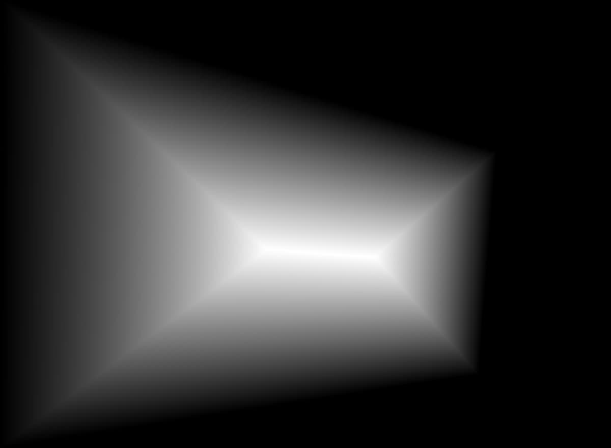
Warped left image on canvas, distance transform mask

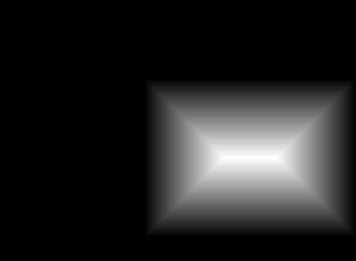
right image on canvas, distance transform mask

Now we have the blending function:

I = \frac{\alpha_1 \cdot I_1 + \alpha_2 \cdot I_2}{\alpha_1 + \alpha_2}

Using the approach above, we get the seamless blending of the two images below. I clipped the new image to be [0, 1] to avoid any overflows.

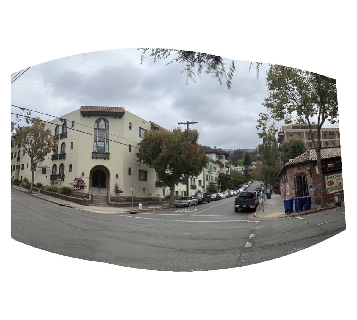
Street mosaic, weighted distance

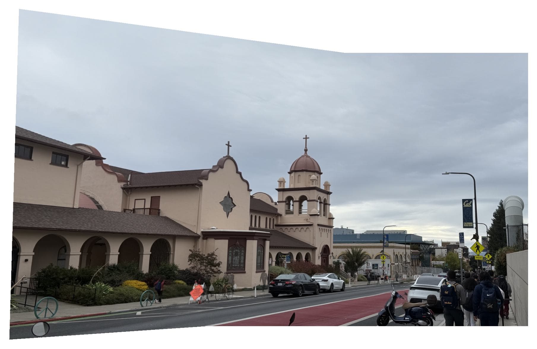
Using the same approach, we can obtain the mosaic of the other two image sets.

Campus (mosaic)

Door (mosaic)

Part A.5: Bells & Whistles

Generate a spherical mosaic: To stitch two images into a spherical panorama, we first need to warp both images onto a common spherical coordinate system. The mapping is done via the following steps:

1. Convert plane coordinates to spherical coordinates: For each image, we map the pixel coordinates $(x, y)$ to spherical angles $(\theta, \phi)$ using a focal length $f$ :

\theta = \arctan\frac{x - c_x}{f}, \quad \phi = \arctan\frac{y - c_y}{f}

where $(c_x, c_y)$ is the image center. This creates a curved projection that simulates a fisheye effect.

2. Compute inverse mapping back to each image: For each pixel on the spherical canvas, we compute the corresponding coordinates in the original images. For the first image:

x_1 = f \cdot \tan(\theta) + c_{x1}, \quad y_1 = \frac{f \cdot \tan(\phi)}{\cos(\theta)} + c_{y1}

and for the second image, we apply the homography $H$ that maps im1 → im2: $\begin{bmatrix} x_2 \\ y_2 \\ 1 \end{bmatrix} = H \begin{bmatrix} x_1 \\ y_1 \\ 1 \end{bmatrix}$ This ensures that features align correctly across the two images.

3. Sample image colors using bilinear interpolation: Using the computed coordinates $(x_1, y_1)$ and $(x_2, y_2)$ , we sample each image using bilinear interpolation.

4. Same approach as flat mosaic: Similar to the flat mosaic, we use distance trasnfrom to smoothly blend two images together, and then combine the warped images using their alpha masks.

The resulting canvas preserves the geometry of each image while applying a spherical effect, and the distance-transform-based alpha masks create smooth blending at the edges.

Street mosaic, sphere mosaic

Campus mosaic, sphere mosaic

Door mosaic, sphere mosaic

B.1: Harris Corner Detection

To perform auto-stitching, we would need to identify a set of features to match from image 1 to image 2. And the first step towards this is to identify interest points in one single image. For this project, we are using the Harris corner detection method, performed on a single scale.

With $\sigma=1$ , the Harris matrix at level $l$ and and position $(x, y)$ is the smoothed outer product of the gradients:

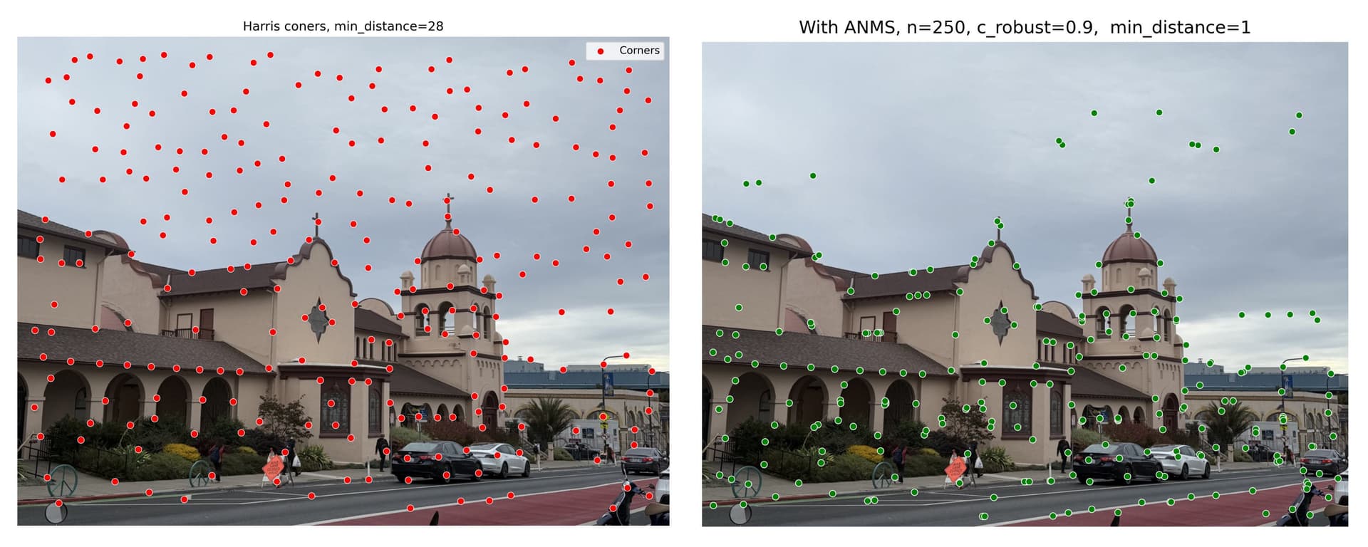
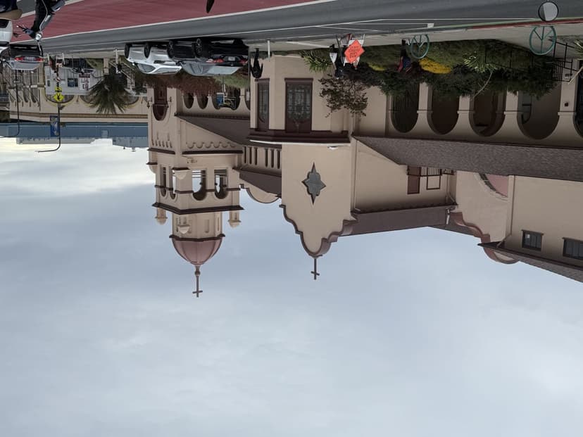
H_l(x, y) = \left( \nabla_{\sigma_d} P_l(x, y) \, \nabla_{\sigma_d} P_l(x, y)^{T} \right) * g_{\sigma_i}(x, y)

With min_distance set to 1, we see that thousands of points are generated on the image. With min_distance=28, the naive Harris corner detection method gives us around 254 points.

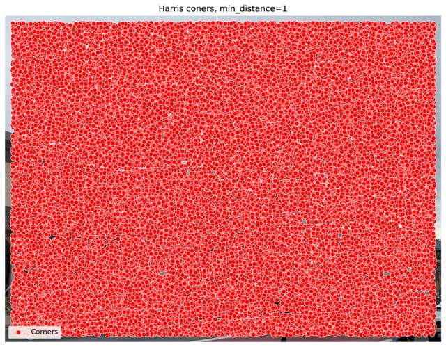
Campus, Harris corners, min_distance=1

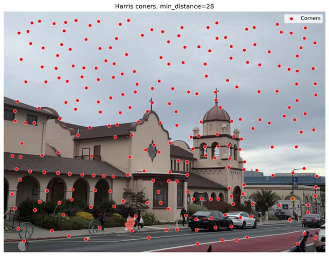
Campus, Harris corners, min_distance=28

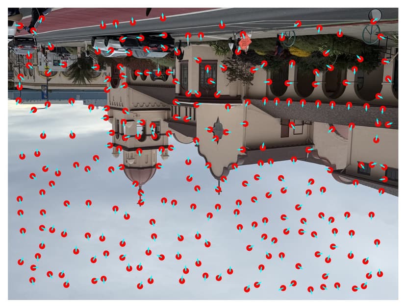
Adaptive non-maximal suppression. The computational cost of matching is superlinear in the number of interest points, using Harris corners. Also, it is important that interest points are spatially well distributed over the image, since the area of overlap between a pair of images may be small for the image stitching case. To reduce computational cost and improve performace, we could use adaptive non-maximal suppression (ANMS) to select a fixed number of interest points from each image.

ANMS essentially suppresses all local harris corners wihtin a range of suppression radius r, unless the point is a local maximum within the suppression radius. Thus the minimum suppression radius $r_i$ is given by

r_i = \min_j \, |x_i - x_j| \quad \text{s.t.} \quad f(x_i) < c_{\text{robust}} f(x_j), \; x_j \in \zeta

where $x_i$ is a 2D interest point image location, and $\zeta$ is the set of all interest point locations. We use a value $c_{robust}$ = 0.9 to ensure that a neighbour must have significantly higher strength for suppression to take place. We select the $n_{ip}$ = 250 interest points with the largest values of $r_i$ .

To avoid ANMS returning local maximum in a flat area (where gradient value approaches 0), I added a threshold so that flatter areas in the image gets artificially large suppression radius. This is effective, as the below ANMS harris corners are all concentrated along the edges and corners of the building, rather than distributed in the sky like the one without using ANMS.

Campus, ANMS comparison

B.2: Feature Descriptor Extraction

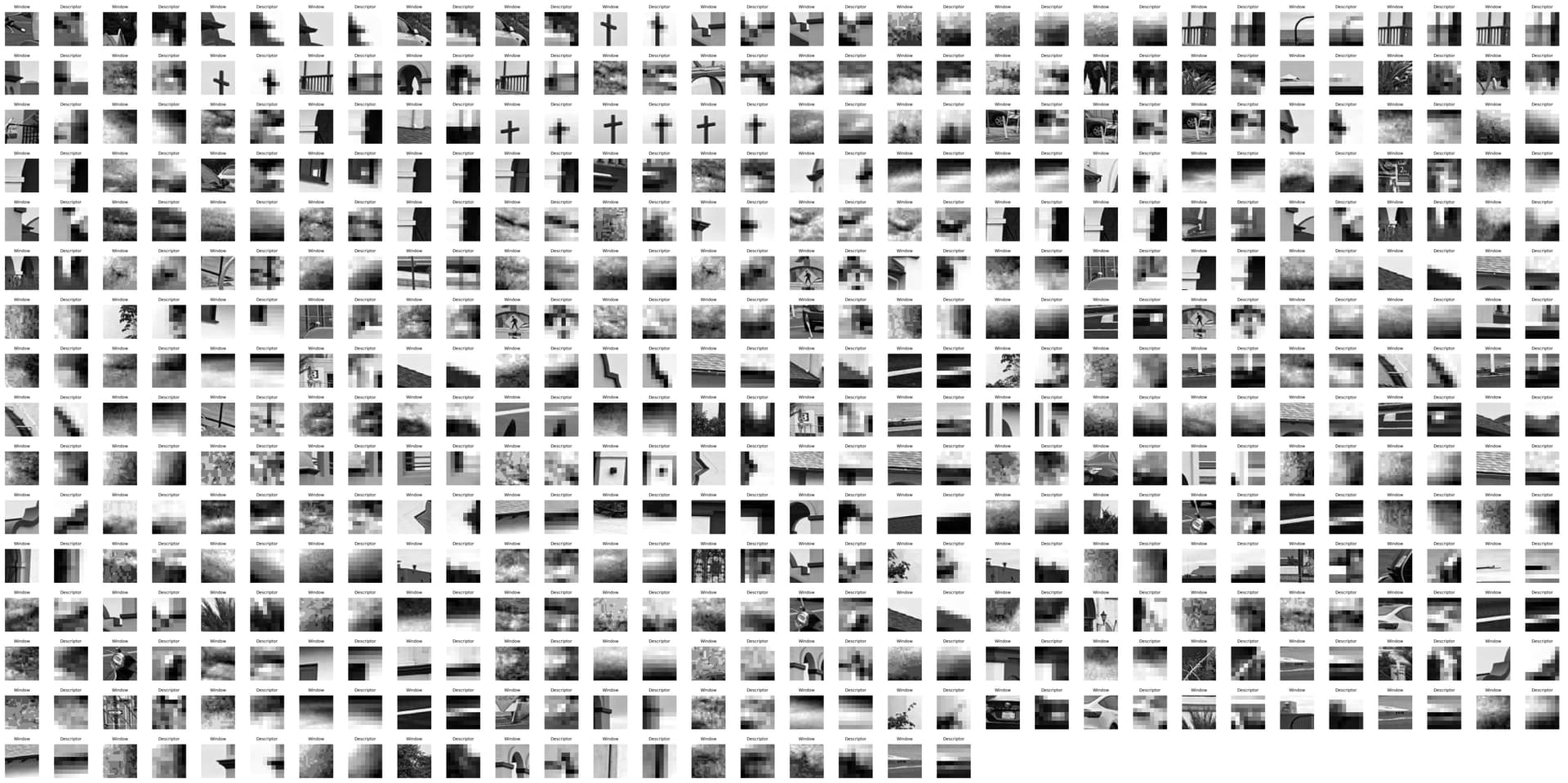
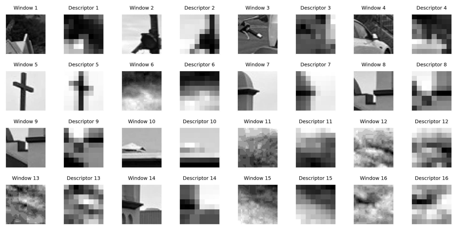
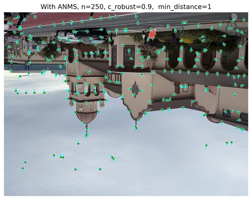
Once we have determined where to place our interest points, we need to extract a description of the local image structure that will support reliable and efficient matching of features across images. A simple way to do that is to first get 40 x 40 window, with each interest point as center. Then we downsample the window by 5 times, so we get an 8 x 8 lower-res patch for each interest points.

After sampling, the descriptor vector is normalised so that the mean is 0 and the standard deviation is 1. This makes the features invariant to affine changes in intensity (bias and gain).

Below is an overview of all 250 normalized feature descriptors, with their corresponding 40x40 window. I have also picked the first 16 descriptors for a more detailed view.

Overview of all 250 descriptors

First 16 descriptors zoomed in

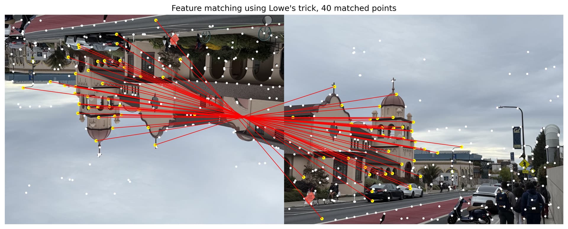
B.3: Feature Matching

Given the patches extracted from the previous step, the goal of the matching stage is to find geometrically consistent feature matches between image pairs. This proceeds as follows. First, we find a set of candidate feature matches using an approximate nearest neighbour algorithm. Then we refine matches using an outlier rejection procedure based on the noise statistics of correct/incorrect matches. This would give us the feature matches in the image pairs.

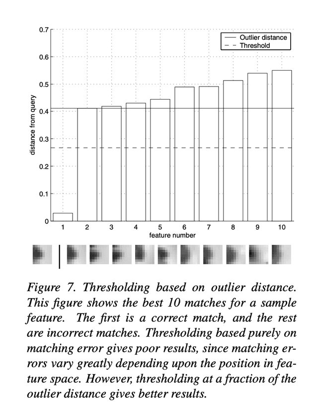
Lowe's trick. Lowe’s ratio test compares the error of the first nearest neighbor (1-NN) to the second nearest neighbor (2-NN) for a given feature. Using the ratio $e_{1 ext{-NN}} / e_{2 ext{-NN}}$ instead of the absolute 1-NN error provides better separation between correct and incorrect matches. This works because correct matches have consistently lower errors than incorrect matches, but the overall error scale varies across features. The 2-NN distance serves as an estimate of the outlier (incorrect match) distance, allowing a discriminative comparison rather than assuming uniform Gaussian noise in feature space.

For this project, I initially set an error threshold threshold_error_nn=0.3, based on rough estimation from the NN-threshold chart in the paper.

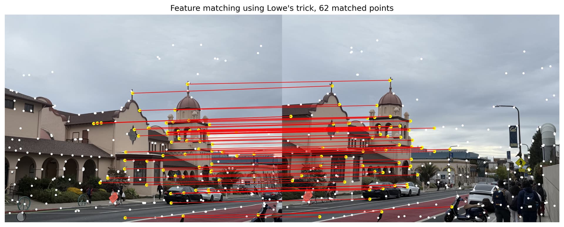
Using the approach above, I obtained matching points for each image pairs as below.

Feature matching for campus

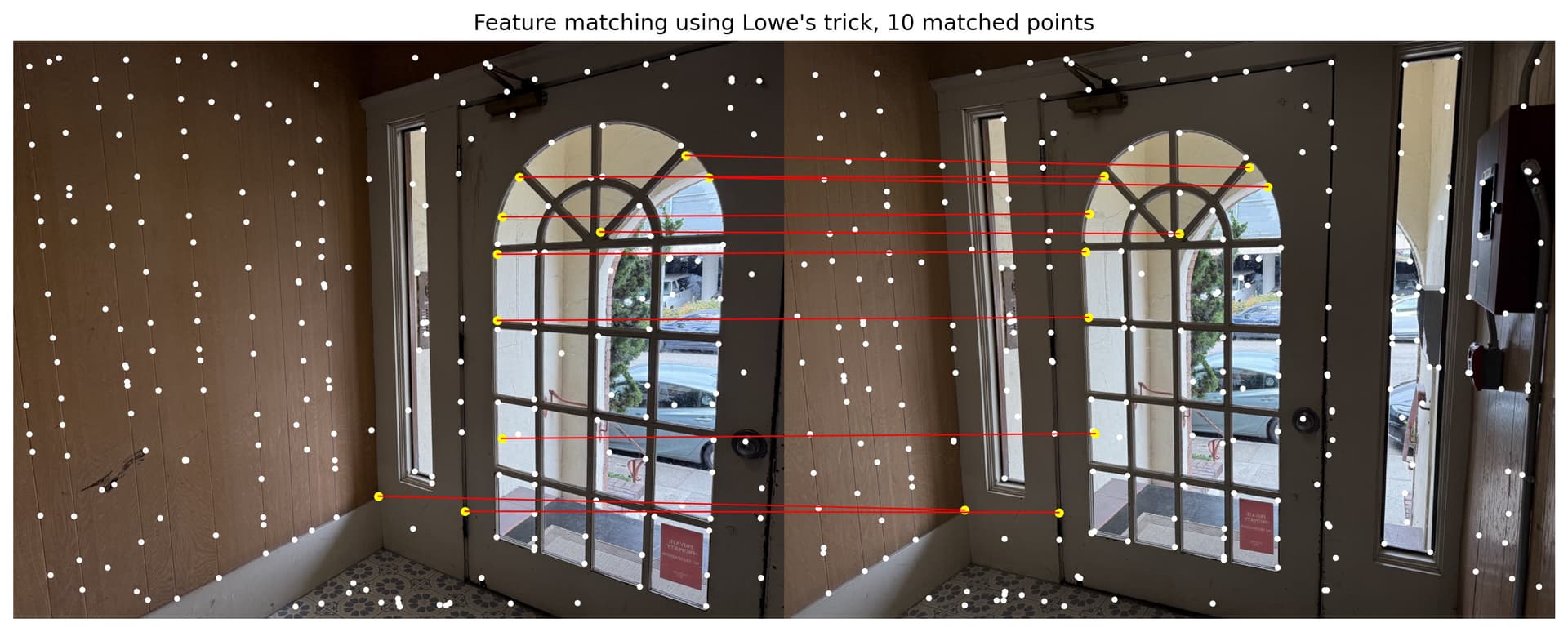
Feature matching for door

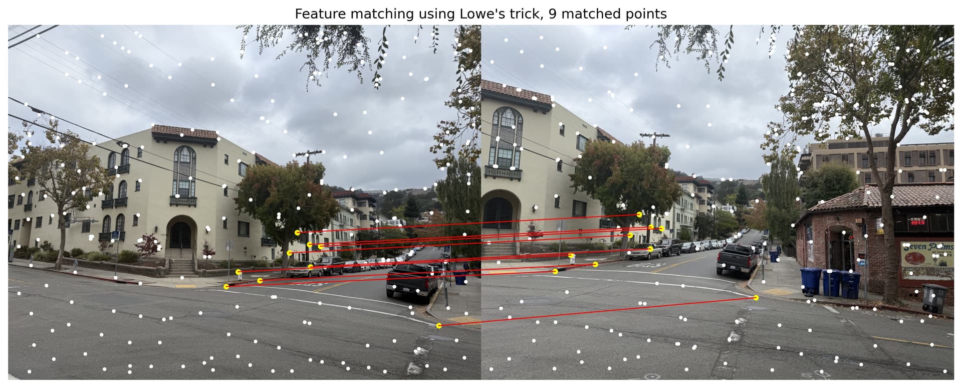
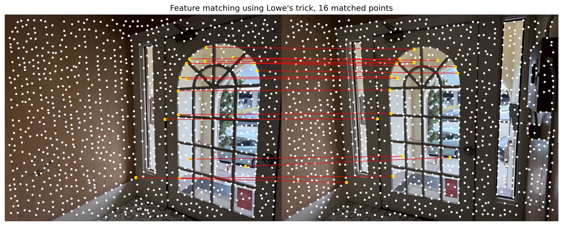
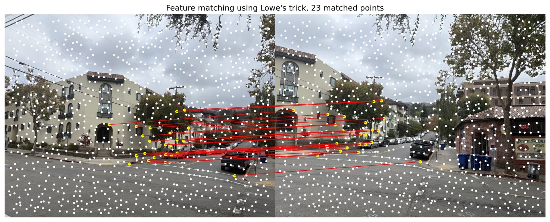
Feature matching for street

B.4: RANSAC for Robust Homography

Now is time to render the auto-stitching images. We use the RANSAC algorithm to create the homography transformation. Below is the RANSAC algorithm I followed to compute robust homography.

Random Sample Consensus (RANSAC) Algorithm:
1. Randomly select 4 pairs of matching feature points.
2. Compute the homography matrix H.
3. Evaluate H on all matches:
a. Define an inlier_threshold to determine if a transformed point is an inlier (i.e., within the threshold distance of its match in image 2).
b. Count the total number of inliers.
4. Keep the H with the highest number of inliers.
5. Repeat for a specified number of iterations.
6. Recompute H using all inliers to obtain the final homography.

The above algorithm has a few parameters, and below are the ones I used for my initial RANSAC computation.

# Number of points sampled from ANMS
num_points=250
# Peak local maximum distance in ANMS
min_distance=1
# Error threshold for nearest neighbor algorithm, threshold = err_1nn / err_2nn
threshold_error_nn=0.3
# RANSAC inliner threshold: range for features to be considered as inliners
inliner_threshold=5
# RANSAC number of iterations
num_iters=1000

Here are the result homographies my RANSAC algorithm produced.

Campus, RANSAC

Door, RANSAC

Street, RANSAC

Comparing manual and auto stitching

Below are side-by-side comparisons between manual and auto stitching. Manual stitching images are from Project 3 part A. We could see that while the campus and door image sets have very similar homography alignment results, manual stiching outperforms auto stitching in the street image set.

Campus, manual stitching

Campus, auto stitching

Door, manual stitching

Door, auto stitching

Street, manual stitching

Street, auto stitching

If you zoom into the street auto-stitching image, you could see blurs on the top right corner of the building.

As one could tell, the RANSAC-computed homography for the campus pair and the door pair are almost perfect, while the street pair is off by obvious error margins. If one look closely to the street homography, the building has some misalignment . Why does this happen, and how could we improve the alignment?

Improvements. This is mostly because the Street image pairs has yielded very few matching points in step B.3. While the campus image set have 62 pairs of points for RANSAC to randomly select from, the street images only had 9 pairs.

To fix this, I tuned the parameters and bumped up number of points significantly, from 250 to 1000, so that each image pairs would have more matching features to perform RANSAC with. I also tuned some other parameters, listed below:

# Number of points sampled from ANMS
num_points=100 # used to be 250
# Peak local maximum distance in ANMS
min_distance=10 # used to be 1
# Error threshold for nearest neighbor algorithm, threshold = err_1nn / err_2nn
threshold_error_nn=0.3 # stayed the same
# RANSAC inliner threshold: range for features to be considered as inliners
inliner_threshold=5 # stayed the same
#RANSAC number of iterations
num_iters=1000 # stayed the same

Door, matching features after tuning

Door, RANSAC after tuning

Street, matching features after tuning

Street, RANSAC, after tuning

Comparison of before and after tuning parameters. We could see from the result that tuning the parameters increased number of matching pairs, and improved the alignment in the homography effect.

Image Pair Name	Num of matching features, before tuning	Num of matching features, after tuning
Door	10 pairs	16 pairs
Campus	9 pairs	23 pairs

Street, RANSAC

Street, RANSAC, after tuning

Part B.5 Bells & Whistles: Rotation invariance

In Part B.3, we took patches axis-aligned with the image, o when the image rotates, your patch (and descriptor) won’t align — hence not rotation invariant. This section will add rotation invariance using the orientation angles for each patch. To test this, let us rotate the left image 180 degrees, so the two source images for the campus set mosaic would look like below.

Campus left

Campus right

Step 1. Compute theta. For each Harris corner $(x, y)^T$ , we compute a dominant orientation $\theta$ . The image is first smoothed with a Gaussian of scale $\sigma_o = 4.5$ , then the gradients $I_x, I_y$ are computed. The orientation is given by $\theta = \arctan2(I_y, I_x)$ , aligning the feature descriptor with the local gradient direction for rotation invariance. Below are the interst points with orientation, using harris corner and ANMS.

Campus, Harris corners with orientation

Campus, Harris + ANMS with orientation

Step 2. Get rotation-invariant descriptors. For each interest point (x, y) with orientation θ, we rotate the coordinate frame around that point by $–\theta$ , before extracting the patch. So instead of taking a 40×40 window aligned with the image axes like Part B.3, we take one aligned with the keypoint’s dominant orientation. That way, no matter how the object rotates in the image, the descriptor remains consistent.

Feature descriptors with rotation invarance

Step 3. Feature matching. We perform feature matching as usual, but because of the orientation-invariant descriptors, we now see matching lines between source interest points intersecting with each other. This means that we are no longer only searching for matching features along the image axes, but we are matching features invariant to image rotation.

Campus, matching features with rotation invarance

Step 4. Compute mosaic. Last but not least, we compute our homography. It looks as expected, proving that rotation of input images does not affect the homography alignment due to the rotation-invariance approeach to feature descriptors.

Campus, auto-stitched mosaid using rotation invarance

Project 3: (Auto)stitching and Photo Mosaics

[due 10/8/2025] Part A: IMAGE WARPING and MOSAICING