Project 4: Neural Radiance Field!

Part 0.1: Calibrating Your Camera

Before building NeRF, we need to collect some image data. I printed out the calibration tags and captured 30 images of these tags using my phone camera, keeping the zoom the same. I made sure to vary the angle and distance of the camera for better results.

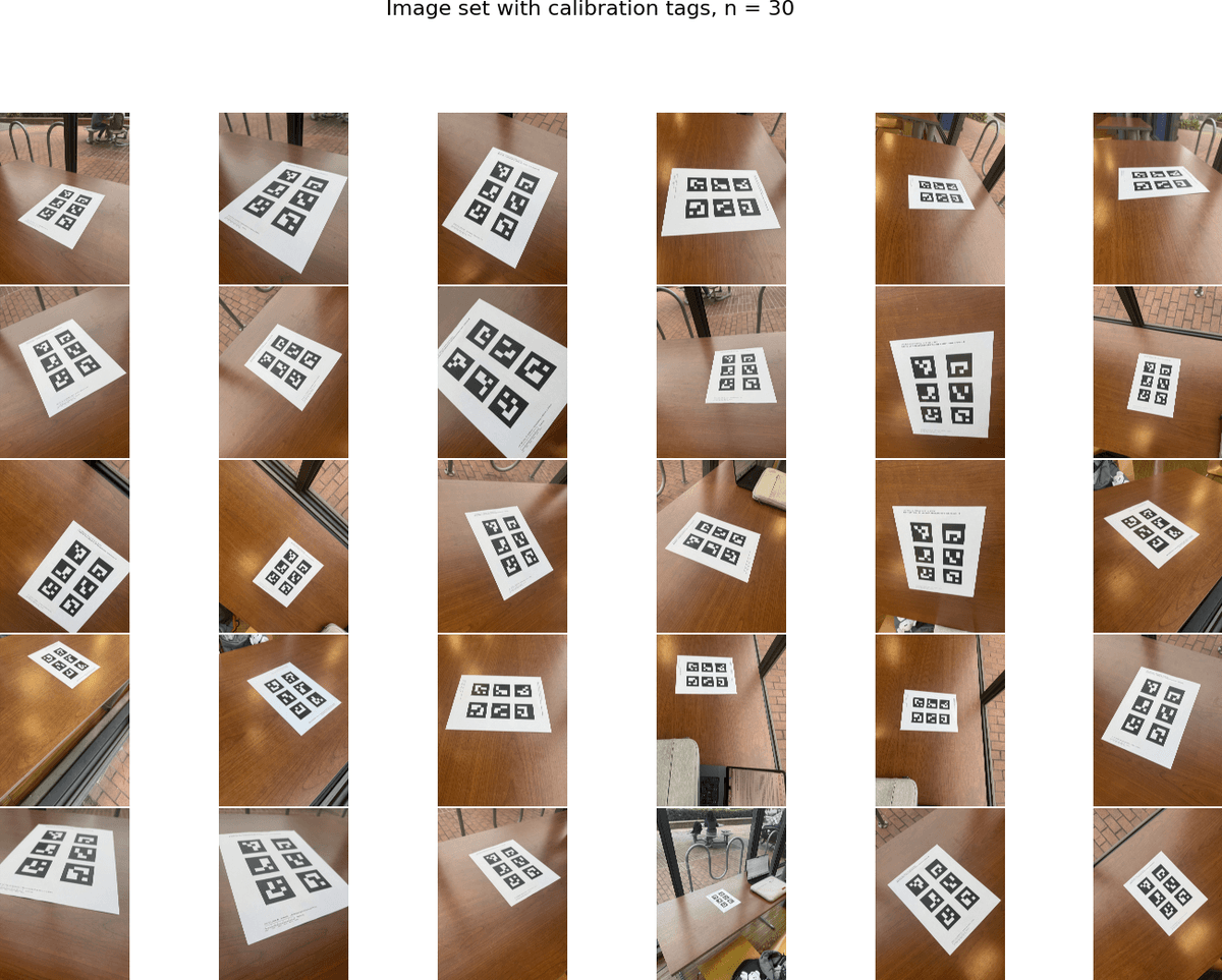
Resizing images from calibration set. Due to the large size of rays and points we are sampling to generate NeRF, I downsampled all of my calibration and training data by 20 times. The images for both the calibration and object sets were (5712, 4284, 3) before resizing, and (285, 214, 3) afterwards. This ensures that the we can run above 5k iterations without worrying about waiting forever.

Camera matrix. To calibrate the camera, I looped through all the calibration images. For each image, I use the OpenCV ArUco detector to Extract the corner coordinates fromall visible tags. To get the 3D world coordinates of the detected corners, I measured the size of each tag and how far they are apart from each other, to compute their world coordinates, assuming the top left corner of the ID=0 tag is (0, 0, 0) in 3D world. I then pass all detected corners and their corresponding 3D world coordinates to cv2.calibrateCamera() to compute the camera intrinsics and distortion coefficients. Below are the values I got for calibrating my phone camera:

Distortion coefficients:

Using the calibration above, I got an RMS reprojection error of 0.25, which is reasonable and within the range of errors for NeRF construciton. This ensures that we don't introduce calibration errors that may yield bad results in the following steps.

Part 0.2: Capturing a 3D Object Scan

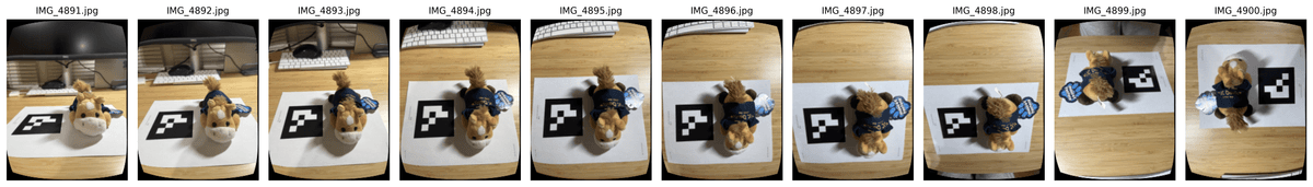
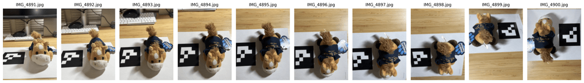
Then, we need to generate an image set of a 3D object. I picked a stuffed animal toy from UC Davis, and placed it next to a single ArUco tag I printed out. Both the tag and the item were on a tabletop. I captured a total of 53 images from different angles, using the same camera and zoom from the previous step. I also made sure to capture images at different andles horizontally and vertically for better rendering, and capturing images at one uniform distance, to ensure better quality of NeRF. Below is the overview of the image dataset.

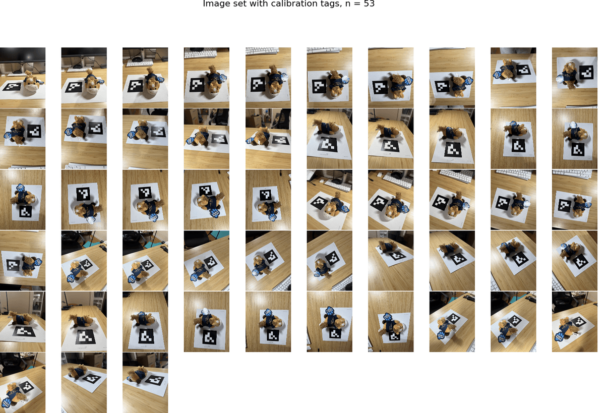
Note that though I captured 53 images, not all images were valid for NeRF, as the stuffed animal blocked the corner of the tag in some images. In such cases, corner detection would fail and my algorithm skips these failed images. In all the steps below, I only used images with valid corner detection for better quality.

Part 0.3: Estimating Camera Pose

For each image in my object scan, I detect the ArUco tag and use cv2.solvePnP() to estimate the camera pose. Similar to Part 0.1, I assume that the origin of the 3D world cooridnates is the top left corner of the tag.

cv2.solvePnP was able to give us the rotation matrix R (from rvec) and translation vector tvec form the camera's extrinsic matrix, which describes where the camera is positioned and oriented relative to the ArUco tag's coordinate system. I then invert this matrix to get the camera-to-world (c2w) matrix for visualization and Part 0.4.

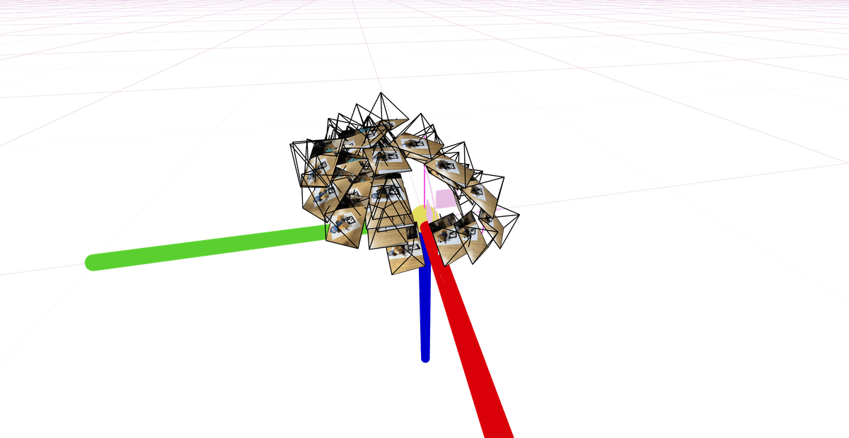
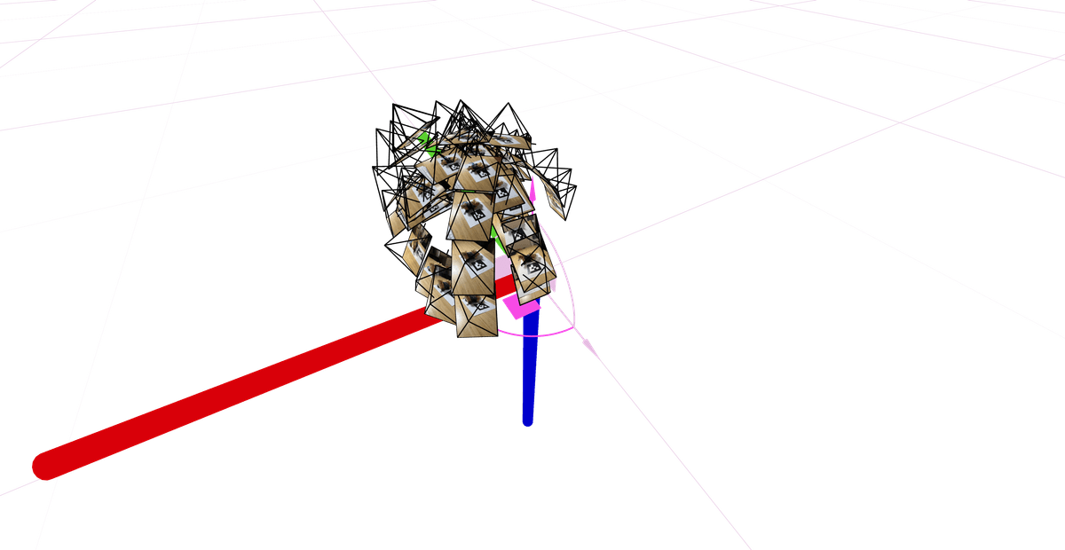
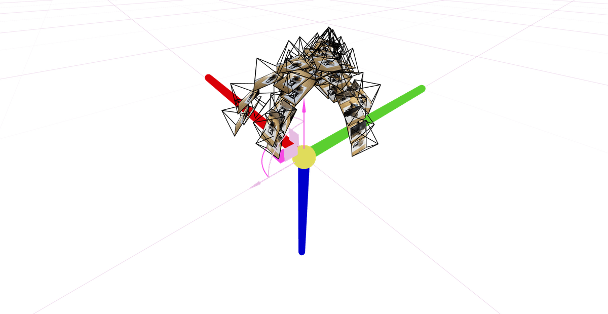
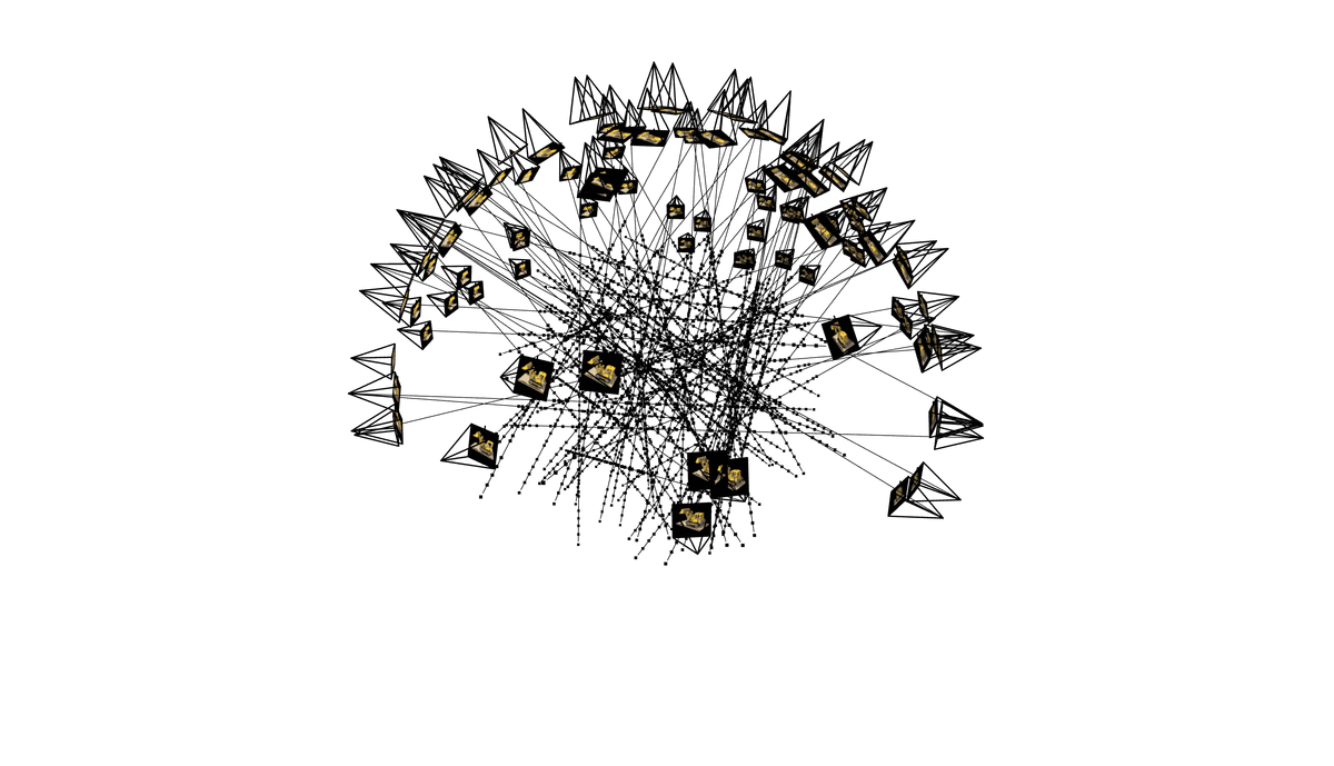
Using Viser and the camera poses we estimated from above, we could see the camera frustums' poses and images to validate the steps so far. Below are some screenshots of my image set visualized with Viser. They form a nice "dome" structure, as I was taking photos of the object from different angles but relatively similar distance.

Part 0.4: Undistorting images and creating a dataset

Since NeRF assumes a perfect pinhole camera model without distortion, we need to undistort the images we took. I used cv2.undistort() to remove any lens distortion from my images, but then I would see black boundaries afterwards.

To fix this, we can use cv2.getOptimalNewCameraMatrix() to compute a new camera matrix that crops out the invalid pixels. See below for the undistortion with and without the optimal new camera matrix, and a side-by-side comparison of the two undistorting approaches.

Undistorted images, calibrated camera matrix

Undistorted images, optimal camera matrix

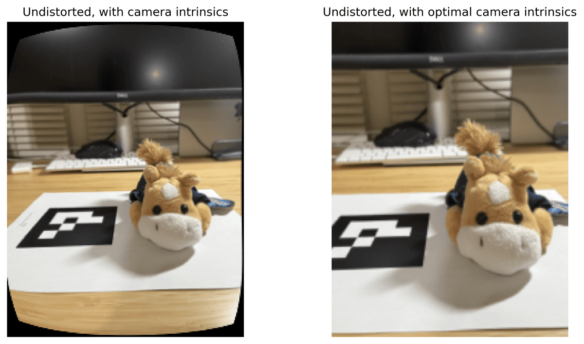
Undistorted comparison

Optimal camera matrix after undistortion. The optimal new camera matrix would be our new camera intrinsics matrix from now on. I stored this new K matrix in my dataset file, along with an 80-10-10 split of my training, validation, and testing data.

Though we could reconstruct the matrix K using focal length and image shape, the optimal camera matrix I obtained here is slightly different from the theoretical reconstructed matrix. For more precise construction of NeRF, I decided to store the optimal camera intrinsics matrix in the dataset file instead.

Part 1: Fit a Neural Field to a 2D Image

Before constructing NeRF, we start with NeRF in 2D. Below are the hyperparameters I used for my MLP, which takes in a 2D coordinate (x, y) and outputs pixel colors in (r, g, b). Before passing the 2D coordinates into the nueral network, I applied sinusoidal Positional Encoding (PE) to the coordinates to expand its dimensionality. PE can expand dimensionality of an 2D input to 2 * (2 * L + 1) dimensions, L being a constant value indicating max frequency. To start, I used the following hyperparameters to train for the 2D NeRF MLP.

layer_width = 256 
L = 10 # max_frequency 
learning_rate = 1e-2

model = nn.Sequential(
    # Linear
    nn.Linear(2 * (2 * L + 1), layer_width),
    # ReLU
    nn.ReLU(),
    # Linear
    nn.Linear(layer_width, layer_width),
    # ReLU
    nn.ReLU(),
    # Linear
    nn.Linear(layer_width, layer_width),
    # ReLU
    nn.ReLU(),
    # Linear
    nn.Linear(layer_width, 3),
    # Sigmoid
    nn.Sigmoid()
)

The above is the architecutre of my MLP. Using the above parameters, with 2k iterations, I was able to get really good output images, with PSNR > 26 during the training iterations.

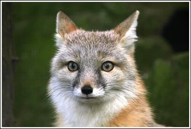
Fox

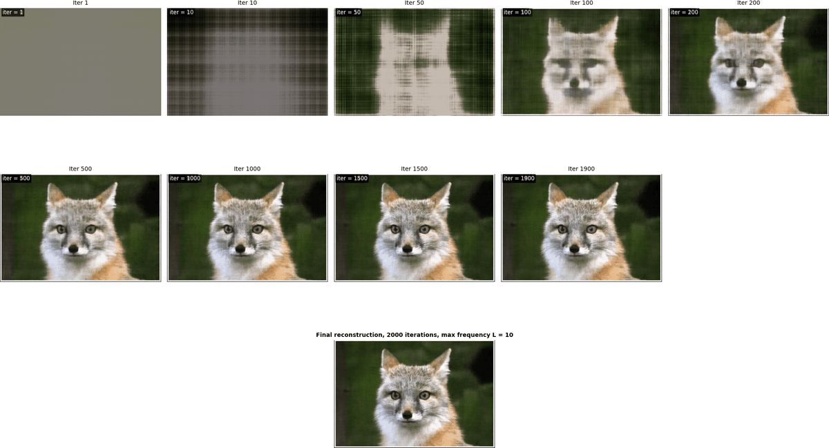
Training progress, fox

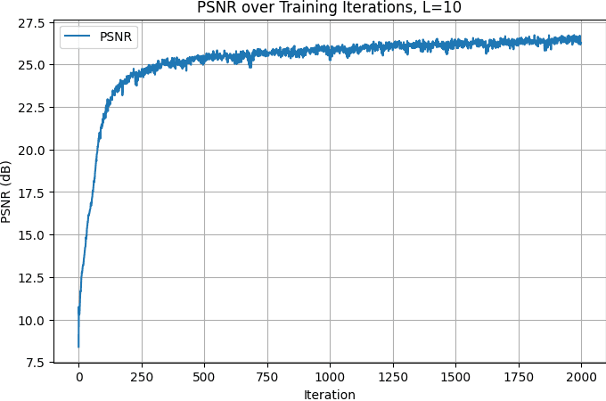
Training PSRN curve, fox

To explore the effect of hyperparameters, I set the positional encoding (PE) maximum frequency and the MLP layer width to very low values. The 2x2 chart below shows their impact on training. With a low PE frequency, the model loses coordinate information, resulting in distorted output features. With a narrow MLP, fine details are lost, while overall structures are maintained, producing lower-resolution images with accurate features.

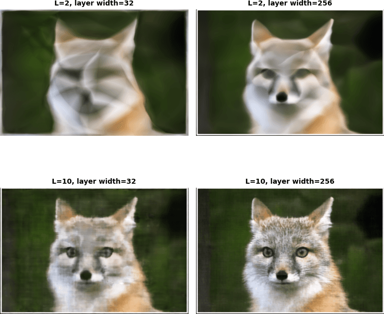
Hyperparameter tuning, fox

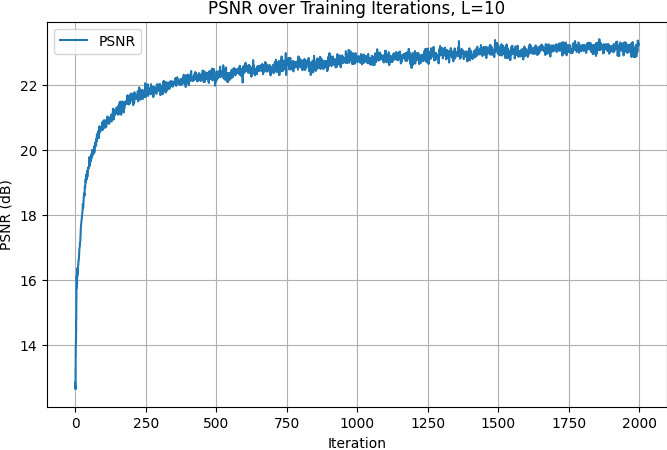
I have also tested this MLP with a random image of my choice. The above is the architecutre of my MLP. Using max frequency = 10, with 2k iterations, I was able to get really good traning PSRN value above 23 here.

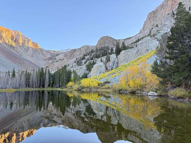
Lake

NeRF quickly captures the overall structure: after just 100 iterations, a rough sketch of the lake view is visible. The remaining ~1900 iterations are spent refining local details.

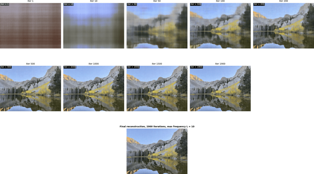
Training progress, lake

Training PSRN curve, lake

Part 2: Fit a Neural Radiance Field from Multi-view Images

Part 2.1: Create Rays from Cameras

To convert points from camera coordinates to world coordinates, I implemented x_w = transform(c2w, x_c), which applies the camera-to-world matrix to homogeneous coordinates. For pixel-to-camera conversion, I inverted the standard projection by implementing x_c = pixel_to_camera(K, uv, s), where $K$ is the intrinsic matrix and $uv$ are the pixel coordinates. Finally, for each pixel, I compute the ray origin $ray_o = c2w[:3,3]$ and the normalized direction $ray_d = \frac{(x_w - ray_o)}{ ||x_w - ray_o||}$ via pixel_to_ray(K, c2w, uv).

All functions above support batched points for efficiency, and I ensured all operations were on cuda for max efficiency.

See detailed implementation of this section in code.

Part 2.2: Sampling

Given rays from Part 2.1, I uniformly sample points along each ray using t = torch.linspace(near, far, N_samples). The actual 3D points are computed as points = ray_o + t * ray_d`. To avoid overfitting and introduce stochasticity during training, I added small perturbations: t = t + (torch.rand_like(t)-0.5) * delta. Rays themselves are sampled either globally across all images or from individual images, by flattening pixels and using random indices, returning ray origins, directions, and corresponding colors.

See detailed implementation of this section in code.

Part 2.3: Putting the Dataloading All Together

I created a RaysDataset class that encapsulates multiview images. I have a sample_rays(N) method to randomly sample N rays and returns (ray_o, ray_d, colors). It internally uses the camera-to-world transformation and pixel-to-ray functions to convert pixel coordinates to rays.

I also implemented sampling functions to sample points from ray and from each camera, for debugging and visualization. i.e. sample_rays_from_camera(cam_idx, N).

I generate points along rays with sample_points_along_rays(ray_o, ray_d, n_samples, near, far, perturb)to feed into the NeRF model.

Below are the visualization of camera poses and the rays we sample

Lego full render

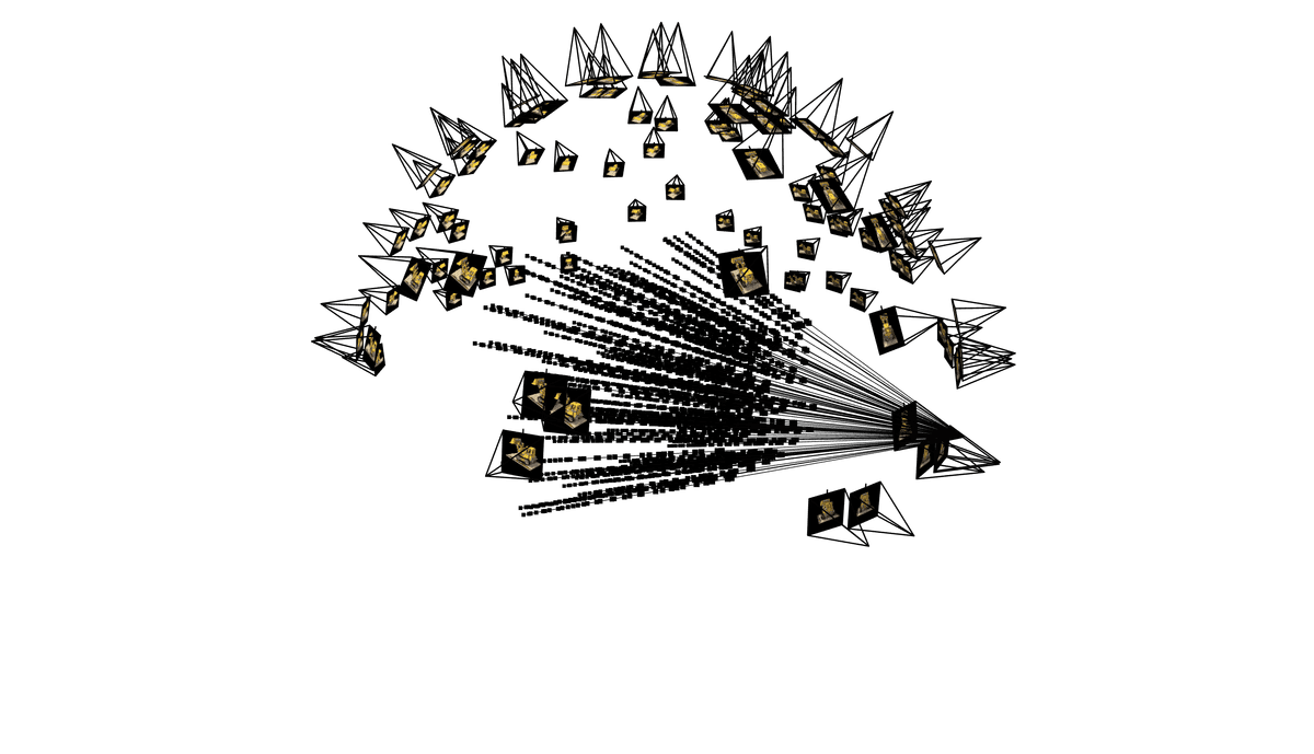
Single camera ray sampling

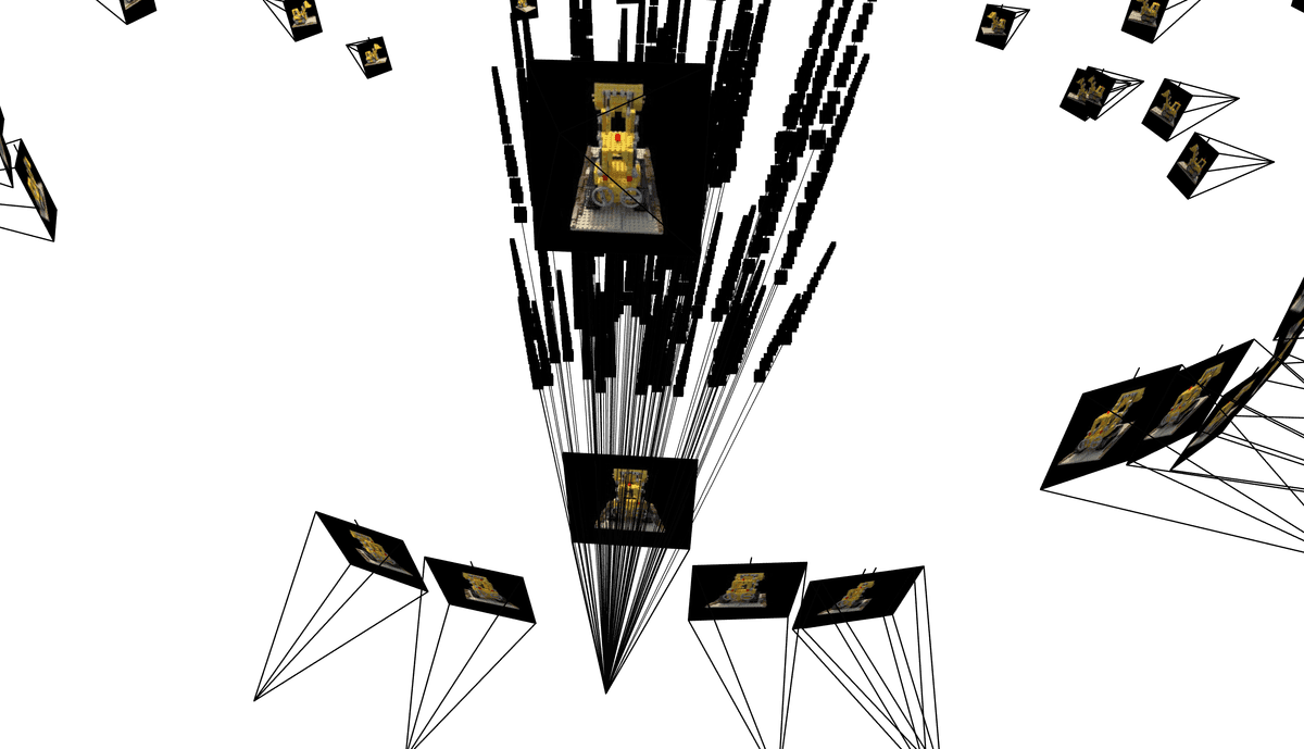
Single camera ray sampling, different angle

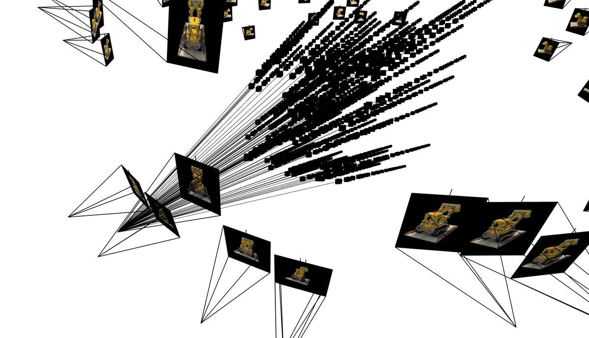
Single camera ray sampling 3, different angle

Part 2.4: Neural Radiance Field + Part 2.5: Volume Rendering

To build NeRF in 3D, I followed the below approach to obtain the density value $\sigma$ and the 3D RGB value of the point sampled on the ray.

Where: $c_i$ is the RGB color predicted by the network at sample i along the ray, $\alpha_i$ is the probability of the ray terminating at sample i, and $T_i = \prod_{j = 1}^{i - 1} (1 - \alpha_j)$ is the probability of the ray not terminating before sample i.

The MLP now processes more information than in Part 1, as it handles multiple samples along many rays from multiple cameras. Its architecture takes the 3D world coordinates of a sampled point and the ray direction as input, and outputs the density sigma and RGB color of that point.

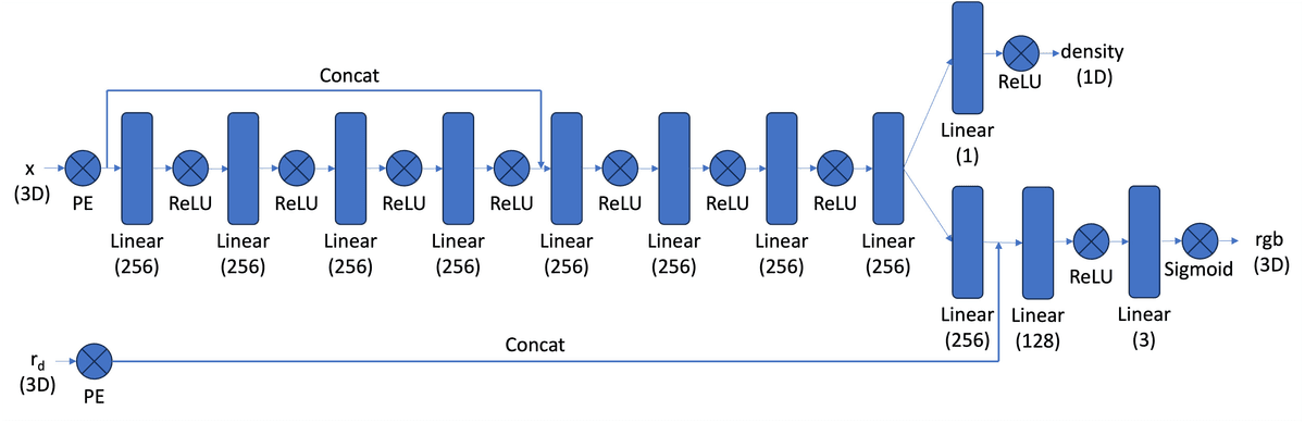
3D NeRF, architecture

With the hyperparameters below, I trained a 3D NeRF on a 200x200 pixels lego image set, and constructed a novel view of the 3D object, with validation PSNR above 23.50.

# training
num_iters = 1500
batch_size = 10000
N_samples = 64
near, far = 2.0, 6.0
lr=5e-4

NeRF, lego

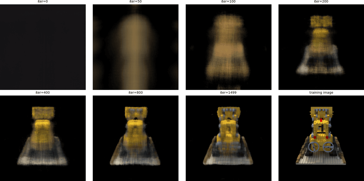
Training progress, lego

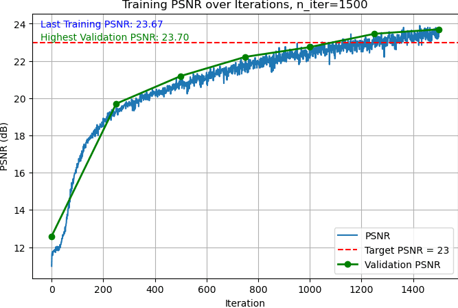
Training and validation PSNR, lego

Bells & Whistles: Construct depth NeRF. To get depth from a NeRF model instead of RGB colors, I still followed the same steps to sample 3D points along each ray between the near and far planes. Then I pass these points and ray directions through the trained NeRF to get densities $\sigma$ and colors, and compute per-sample alpha $\alpha = 1 - e^{-\sigma \Delta}$ and calculate weights along each ray using cumulative transmittance. All the steps till here are the same as constructing an RGB NeRF. But to compute the depth for each ray, I computed the expected depth for each ray as the weighted sum of the sample depths: $\text{depth} = \sum_i w_i z_i$, where $z_i$ are the distances of the sampled points along the ray. Reshape the resulting depth array to match the image dimensions for visualization.

NeRF Depth, lego

Part 2.6: Training with your own data

In this section, I first used the Lafufu Dataset to debug and validate that my camera poses and estimations from Part 0 is correct. Then, I used my own dataset, a stuffed animal toy from UC Davis, to render NeRF. I also built a function to construct 360-degree orbit animation to visualize NeRF results.

Visualize 3D reconstruction: orbit animation. To visualize the 3D reconstruction from the NeRF model, I generated 360-degree orbit animations of the object. I first pick a few "good" images from the dataset, and use their camera-to-world matrices to construct the orbiting animation.

For each selected base camera from the dataset, I computed the vector from the object center to the camera and rotated this vector around the world Z-axis to simulate a circular camera path around the object. At each rotated position, the camera was oriented to look directly at the object center, ensuring it remained in view. The network then rendered images from these virtual camera poses, which were combined into frames in GIFs to show the object from all angles.

Out of all the "good" images I picked to generate the gifs, I go through the gifs and pick one that has the most coverage of the angles to display. The 360-degree orbit animation helps visualize the quality of the reconstruction and the geometric relationships from different viewpoints are preserved.

Lafufu Dataset

Below is a quick validation, using Lafufu training data for traning the NeRF network after 3000 iterations, and the validation data for geneating this video below.

# Lafufu training
num_iters = 3000
batch_size = 10000
N_samples = 64
near, far = 0.02, 0.5
lr=5e-4

For 3k iterations, I was able to reach around 18-20 PSNR using the Lafufu dataset. This was a confirmation that my MLP was indeed learning and generting pixel values that are on the right track. I was then ready to generate my own NeRF.

NeRF, Lafufu Dataset

My own dataset

Below are the analysis for generating NeRF using my own Davis Dataset. I picked the same near and far values for my Davis dataset as the Lafufu one, because I took the photos for the Davis dataset pretty closely to the object, just as how the Lafufu dataset was constructed.

# My own dataset training
num_iters = 5000
batch_size = 10000
N_samples = 64
near, far = 0.02, 0.5
lr=5e-4

For my custom dataset training, I consistently keep N_samples = 64 for discretizing each ray. This ensures a sufficiently dense sampling along the ray for accurate volume rendering while keeping memory usage manageable. At each training iteration, I sample batch_size = 10000 rays from the dataset, which allows the model to see a diverse set of points across multiple views and accelerates convergence. Based on my experiments, smaller samples of rays or batch size do not yield good result.

NeRF, Davis Dataset

Note for data quality improvement. Looking at the GIF above, it's unfortunate that the object is partially outside the image in some frames. If I were to collect the data again, I would choose a smaller item and/or put my phone horizontally to capture the images. As the above GIF shows, during 3D reconstruction, the object sometimes moves out of frame during rotation. This shows a key limitation of NeRF reconstruction: the model relies heavily on consistent coverage of the object from all angles. If parts of the object are not captured in the dataset, the network cannot fully reconstruct them, leading to incomplete or unstable geometry in certain views. If I framed my camera more carefully, the data quality would have been better for reconstruction.

Below is the visualization of the training progress, using an arbitrary image from the dataset. As mentioned above, the later iterations focus on refining local details, while the ealry iterations get the rough sketches of the image pretty quickly.

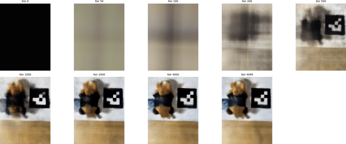
NeRF training progress visualized, Davis Dataset

I was able to achieve above 23.50 PSNR for the training dataset, and above 20 PSNR for the validation set.

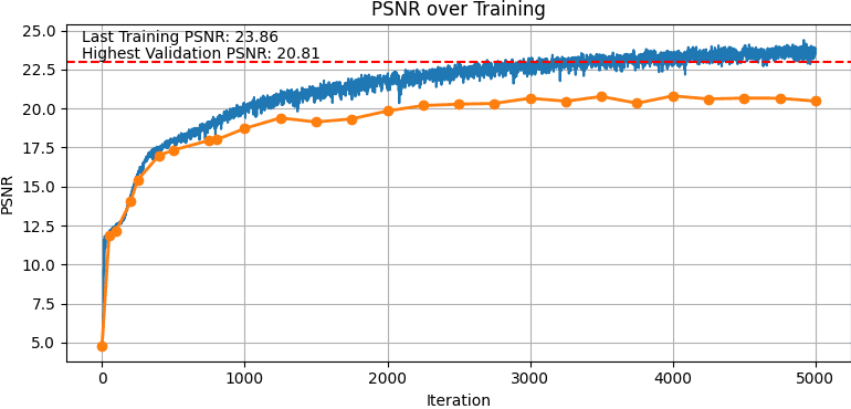
NeRF PSNR for training and validation, Davis Dataset

The training loss steadily drops over time as the model learns to match the ground-truth pixel colors. Early in training, the loss decreases rapidly as NeRF captures the coarse structure of the scene. As iterations continue, the curve flattens, reflecting slower but steady improvements as the network focuses on refining fine details and reducing small color discrepancies.

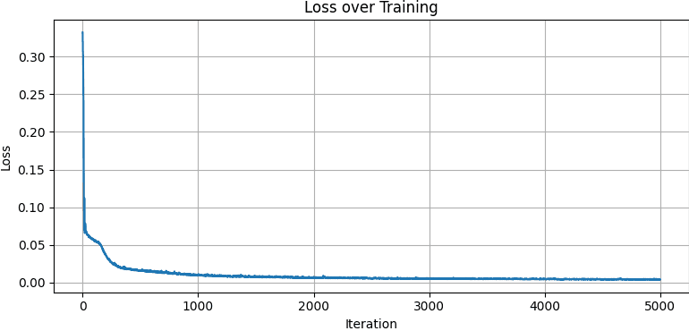
NeRF training loss, Davis Dataset