Project 5: Fun With Diffusion Models!

Part 0: Setup

I decided to come up with three pairs (six in total) of prompts, each describing one object. Within each pair, I use one short prompt that is very concise, and one longer prompt that goes into details on the object. Below are the prompts I used:

A cat riding a motorcycle.

Dreamlike surrealist painting style. A cat with translucent pastel tentacles and riding a motorcycle. Blended gradients, ethereal glow, painterly brush textures. Transparent background, centered.

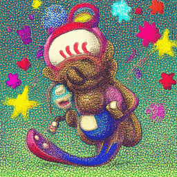
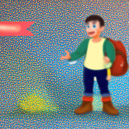
A 2D cartoon character.

2D animated, warm and inviting cartoon character in soft pastel colors, flat-vector style. Ethnically neutral, gender-neutral, wearing casual outdoorsy clothes with a backpack. One hand raised in a friendly wave, light gentle smile, relaxed and welcoming posture. Green hoodie, dark blue pants, brown boots, yellow backpack. Eyes looking forward naturally. Clean smooth lines, minimal brush strokes, subtle shading, harmonious warm tones, cozy and playful feel, crisp edges, polished and simple, transparent background, full body, centered, game-ready style for animation sprites.

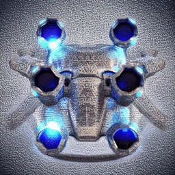
A sci-fi drone.

High-detail 3D sci-fi drone rendered in sleek hard-surface style. Metallic cool-tone palette (steel, gunmetal, silver) with subtle emissive blue accents. Compact spherical body with symmetrical quad rotors, glowing energy core at the center. Sharp, precise edges and reflective surfaces. Industrial-futuristic aesthetic inspired by AAA game concept art. Dynamic but stable hover pose. Soft studio lighting, crisp shadows, photorealistic reflections. No background (transparent), clean polished finish, centered, full object, production-ready for robotics concept visualization.

With seed = 100 and num_inference_steps = 20, I picked three prompts and generated images using the DeepFloyd model.

stage 1: A 2D cartoon character.

A 2D cartoon character.

stage 1: 2D animated, warm and inviting cartoon character in soft pastel colors, flat-vector style. Ethnically neutral, gender-neutral, wearing casual outdoorsy clothes with a backpack. One hand raised in a friendly wave, light gentle smile, relaxed and welcoming posture. Green hoodie, dark blue pants, brown boots, yellow backpack. Eyes looking forward naturally. clean smooth lines, minimal brush strokes, subtle shading, harmonious warm tones, cozy and playful feel, crisp edges, polished and simple, transparent background, full body, centered, game-ready style for animation sprites.

2D animated, warm and inviting cartoon character in soft pastel colors, flat-vector style. Ethnically neutral, gender-neutral, wearing casual outdoorsy clothes with a backpack. One hand raised in a friendly wave, light gentle smile, relaxed and welcoming posture. Green hoodie, dark blue pants, brown boots, yellow backpack. Eyes looking forward naturally. clean smooth lines, minimal brush strokes, subtle shading, harmonious warm tones, cozy and playful feel, crisp edges, polished and simple, transparent background, full body, centered, game-ready style for animation sprites.

stage 1: High-detail 3D sci-fi drone rendered in sleek hard-surface style. Metallic cool-tone palette (steel, gunmetal, silver) with subtle emissive blue accents. Compact spherical body with symmetrical quad rotors, glowing energy core at the center. Sharp, precise edges and reflective surfaces. Industrial-futuristic aesthetic inspired by AAA game concept art. Dynamic but stable hover pose. Soft studio lighting, crisp shadows, photorealistic reflections. No background (transparent), clean polished finish, centered, full object, production-ready for robotics concept visualization.

High-detail 3D sci-fi drone rendered in sleek hard-surface style. Metallic cool-tone palette (steel, gunmetal, silver) with subtle emissive blue accents. Compact spherical body with symmetrical quad rotors, glowing energy core at the center. Sharp, precise edges and reflective surfaces. Industrial-futuristic aesthetic inspired by AAA game concept art. Dynamic but stable hover pose. Soft studio lighting, crisp shadows, photorealistic reflections. No background (transparent), clean polished finish, centered, full object, production-ready for robotics concept visualization.

stage 2: A 2D cartoon character.

A 2D cartoon character.

stage 2: 2D animated, warm and inviting cartoon character in soft pastel colors, flat-vector style. Ethnically neutral, gender-neutral, wearing casual outdoorsy clothes with a backpack. One hand raised in a friendly wave, light gentle smile, relaxed and welcoming posture. Green hoodie, dark blue pants, brown boots, yellow backpack. Eyes looking forward naturally. clean smooth lines, minimal brush strokes, subtle shading, harmonious warm tones, cozy and playful feel, crisp edges, polished and simple, transparent background, full body, centered, game-ready style for animation sprites.

2D animated, warm and inviting cartoon character in soft pastel colors, flat-vector style. Ethnically neutral, gender-neutral, wearing casual outdoorsy clothes with a backpack. One hand raised in a friendly wave, light gentle smile, relaxed and welcoming posture. Green hoodie, dark blue pants, brown boots, yellow backpack. Eyes looking forward naturally. clean smooth lines, minimal brush strokes, subtle shading, harmonious warm tones, cozy and playful feel, crisp edges, polished and simple, transparent background, full body, centered, game-ready style for animation sprites.

stage 2: High-detail 3D sci-fi drone rendered in sleek hard-surface style. Metallic cool-tone palette (steel, gunmetal, silver) with subtle emissive blue accents. Compact spherical body with symmetrical quad rotors, glowing energy core at the center. Sharp, precise edges and reflective surfaces. Industrial-futuristic aesthetic inspired by AAA game concept art. Dynamic but stable hover pose. Soft studio lighting, crisp shadows, photorealistic reflections. 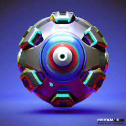No background (transparent), clean polished finish, centered, full object, production-ready for robotics concept visualization.

High-detail 3D sci-fi drone rendered in sleek hard-surface style. Metallic cool-tone palette (steel, gunmetal, silver) with subtle emissive blue accents. Compact spherical body with symmetrical quad rotors, glowing energy core at the center. Sharp, precise edges and reflective surfaces. Industrial-futuristic aesthetic inspired by AAA game concept art. Dynamic but stable hover pose. Soft studio lighting, crisp shadows, photorealistic reflections. No background (transparent), clean polished finish, centered, full object, production-ready for robotics concept visualization.

The examples above were generated with num_inference_steps = 20. I also experimented with num_inference_steps = 5 and 100. Below are the results for num_inference_steps = 5. Compared to num_inference_steps = 20, the generated images appear rougher and less refined. While they still follow the prompts, the backgrounds exhibit more noise and artifacts, indicating that fewer inference steps reduce the quality of the final output.

stage 1: A 2D cartoon character.

A 2D cartoon character.

stage 1: 2D animated, warm and inviting cartoon character in soft pastel colors, flat-vector style. Ethnically neutral, gender-neutral, wearing casual outdoorsy clothes with a backpack. One hand raised in a friendly wave, light gentle smile, relaxed and welcoming posture. Green hoodie, dark blue pants, brown boots, yellow backpack. Eyes looking forward naturally. clean smooth lines, minimal brush strokes, subtle shading, harmonious warm tones, cozy and playful feel, crisp edges, polished and simple, transparent background, full body, centered, game-ready style for animation sprites.

2D animated, warm and inviting cartoon character in soft pastel colors, flat-vector style. Ethnically neutral, gender-neutral, wearing casual outdoorsy clothes with a backpack. One hand raised in a friendly wave, light gentle smile, relaxed and welcoming posture. Green hoodie, dark blue pants, brown boots, yellow backpack. Eyes looking forward naturally. clean smooth lines, minimal brush strokes, subtle shading, harmonious warm tones, cozy and playful feel, crisp edges, polished and simple, transparent background, full body, centered, game-ready style for animation sprites.

stage 1: High-detail 3D sci-fi drone rendered in sleek hard-surface style. Metallic cool-tone palette (steel, gunmetal, silver) with subtle emissive blue accents. Compact spherical body with symmetrical quad rotors, glowing energy core at the center. Sharp, precise edges and reflective surfaces. Industrial-futuristic aesthetic inspired by AAA game concept art. Dynamic but stable hover pose. Soft studio lighting, crisp shadows, photorealistic reflections. No background (transparent), clean polished finish, centered, full object, production-ready for robotics concept visualization.

High-detail 3D sci-fi drone rendered in sleek hard-surface style. Metallic cool-tone palette (steel, gunmetal, silver) with subtle emissive blue accents. Compact spherical body with symmetrical quad rotors, glowing energy core at the center. Sharp, precise edges and reflective surfaces. Industrial-futuristic aesthetic inspired by AAA game concept art. Dynamic but stable hover pose. Soft studio lighting, crisp shadows, photorealistic reflections. No background (transparent), clean polished finish, centered, full object, production-ready for robotics concept visualization.

stage 2: A 2D cartoon character.

A 2D cartoon character.

stage 2: 2D animated, warm and inviting cartoon character in soft pastel colors, flat-vector style. Ethnically neutral, gender-neutral, wearing casual outdoorsy clothes with a backpack. One hand raised in a friendly wave, light gentle smile, relaxed and welcoming posture. Green hoodie, dark blue pants, brown boots, yellow backpack. Eyes looking forward naturally. clean smooth lines, minimal brush strokes, subtle shading, harmonious warm tones, cozy and playful feel, crisp edges, polished and simple, transparent background, full body, centered, game-ready style for animation sprites.

2D animated, warm and inviting cartoon character in soft pastel colors, flat-vector style. Ethnically neutral, gender-neutral, wearing casual outdoorsy clothes with a backpack. One hand raised in a friendly wave, light gentle smile, relaxed and welcoming posture. Green hoodie, dark blue pants, brown boots, yellow backpack. Eyes looking forward naturally. clean smooth lines, minimal brush strokes, subtle shading, harmonious warm tones, cozy and playful feel, crisp edges, polished and simple, transparent background, full body, centered, game-ready style for animation sprites.

stage 2: High-detail 3D sci-fi drone rendered in sleek hard-surface style. Metallic cool-tone palette (steel, gunmetal, silver) with subtle emissive blue accents. Compact spherical body with symmetrical quad rotors, glowing energy core at the center. Sharp, precise edges and reflective surfaces. Industrial-futuristic aesthetic inspired by AAA game concept art. Dynamic but stable hover pose. Soft studio lighting, crisp shadows, photorealistic reflections. No background (transparent), clean polished finish, centered, full object, production-ready for robotics concept visualization.

High-detail 3D sci-fi drone rendered in sleek hard-surface style. Metallic cool-tone palette (steel, gunmetal, silver) with subtle emissive blue accents. Compact spherical body with symmetrical quad rotors, glowing energy core at the center. Sharp, precise edges and reflective surfaces. Industrial-futuristic aesthetic inspired by AAA game concept art. Dynamic but stable hover pose. Soft studio lighting, crisp shadows, photorealistic reflections. No background (transparent), clean polished finish, centered, full object, production-ready for robotics concept visualization.

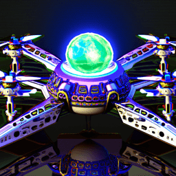
For num_inference_steps = 100, the generation process took significantly longer than the previous examples. The images produced are noticeably more refined and highly detailed. In the drone image, for example, we can even observe the reflection of the drone on the table, demonstrating the improved realism and fidelity achieved with more inference steps.

stage 1: A 2D cartoon character.

A 2D cartoon character.

stage 1: 2D animated, warm and inviting cartoon character in soft pastel colors, flat-vector style. Ethnically neutral, gender-neutral, wearing casual outdoorsy clothes with a backpack. One hand raised in a friendly wave, light gentle smile, relaxed and welcoming posture. Green hoodie, dark blue pants, brown boots, yellow backpack. Eyes looking forward naturally. clean smooth lines, minimal brush strokes, subtle shading, harmonious warm tones, cozy and playful feel, crisp edges, polished and simple, transparent background, full body, centered, game-ready style for animation sprites.

2D animated, warm and inviting cartoon character in soft pastel colors, flat-vector style. Ethnically neutral, gender-neutral, wearing casual outdoorsy clothes with a backpack. One hand raised in a friendly wave, light gentle smile, relaxed and welcoming posture. Green hoodie, dark blue pants, brown boots, yellow backpack. Eyes looking forward naturally. clean smooth lines, minimal brush strokes, subtle shading, harmonious warm tones, cozy and playful feel, crisp edges, polished and simple, transparent background, full body, centered, game-ready style for animation sprites.

stage 1: High-detail 3D sci-fi drone rendered in sleek hard-surface style. Metallic cool-tone palette (steel, gunmetal, silver) with subtle emissive blue accents. Compact spherical body with symmetrical quad rotors, glowing energy core at the center. Sharp, precise edges and reflective surfaces. Industrial-futuristic aesthetic inspired by AAA game concept art. Dynamic but stable hover pose. Soft studio lighting, crisp shadows, photorealistic reflections. No background (transparent), clean polished finish, centered, full object, production-ready for robotics concept visualization.

High-detail 3D sci-fi drone rendered in sleek hard-surface style. Metallic cool-tone palette (steel, gunmetal, silver) with subtle emissive blue accents. Compact spherical body with symmetrical quad rotors, glowing energy core at the center. Sharp, precise edges and reflective surfaces. Industrial-futuristic aesthetic inspired by AAA game concept art. Dynamic but stable hover pose. Soft studio lighting, crisp shadows, photorealistic reflections. No background (transparent), clean polished finish, centered, full object, production-ready for robotics concept visualization.

stage 2: A 2D cartoon character.

A 2D cartoon character.

stage 2: 2D animated, warm and inviting cartoon character in soft pastel colors, flat-vector style. Ethnically neutral, gender-neutral, wearing casual outdoorsy clothes with a backpack. One hand raised in a friendly wave, light gentle smile, relaxed and welcoming posture. Green hoodie, dark blue pants, brown boots, yellow backpack. Eyes looking forward naturally. clean smooth lines, minimal brush strokes, subtle shading, harmonious warm tones, cozy and playful feel, crisp edges, polished and simple, transparent background, full body, centered, game-ready style for animation sprites.

2D animated, warm and inviting cartoon character in soft pastel colors, flat-vector style. Ethnically neutral, gender-neutral, wearing casual outdoorsy clothes with a backpack. One hand raised in a friendly wave, light gentle smile, relaxed and welcoming posture. Green hoodie, dark blue pants, brown boots, yellow backpack. Eyes looking forward naturally. clean smooth lines, minimal brush strokes, subtle shading, harmonious warm tones, cozy and playful feel, crisp edges, polished and simple, transparent background, full body, centered, game-ready style for animation sprites.

stage 2: High-detail 3D sci-fi drone rendered in sleek hard-surface style. Metallic cool-tone palette (steel, gunmetal, silver) with subtle emissive blue accents. Compact spherical body with symmetrical quad rotors, glowing energy core at the center. Sharp, precise edges and reflective surfaces. Industrial-futuristic aesthetic inspired by AAA game concept art. Dynamic but stable hover pose. Soft studio lighting, crisp shadows, photorealistic reflections. No background (transparent), clean polished finish, centered, full object, production-ready for robotics concept visualization.

High-detail 3D sci-fi drone rendered in sleek hard-surface style. Metallic cool-tone palette (steel, gunmetal, silver) with subtle emissive blue accents. Compact spherical body with symmetrical quad rotors, glowing energy core at the center. Sharp, precise edges and reflective surfaces. Industrial-futuristic aesthetic inspired by AAA game concept art. Dynamic but stable hover pose. Soft studio lighting, crisp shadows, photorealistic reflections. No background (transparent), clean polished finish, centered, full object, production-ready for robotics concept visualization.

1.1 Implementing the Forward Process

A key part of diffusion is the forward process, which takes a clean image $x_0$and adds noise to it. The forward process is defined by:

which is equivalent to computing

That is, given a clean image $x_0$, we get a noisy image $x_t$ at timestep $t$ by sampling from a Gaussian with mean $\sqrt{\bar{\alpha}_t}x_0$ and variance $1 - \bar{\alpha}_t$.

Using the Berkeley Campanile image and the forward function, below are the Campanile at noise level [250, 500, 750]. We observe an increasing amount of noise pixels in the images as noise level goes up.

Berkeley Campanile

Noisy Campanile at t=250

Noisy Campanile at t=500

Noisy Campanile at t=750

1.2 Classical Denoising

Here, we are using Gaussina blur filtering to try to remove the noise from the noisy images generated above. We observe that the noisy images are blurry, but the Guassian does not successfully remove the noise here.

Noisy Campanile at t=250

Noisy Campanile at t=500

Noisy Campanile at t=750

Gaussian Blur Denoising at t=250

Gaussian Blur Denoising at t=500

Gaussian Blur Denoising at t=750

1.3 One-Step Denoising

Now, we use a pretrained diffusion model stage_1.unet to denoise, by recovering Gaussian noise from the image and removing this noise to recover the original image.

First, we use the forward() function to add noise to the original image. Then, we estimate the noise in the new noisy image by passing it through the diffusion model stage_1.unet. This noise is the $\epsilon$ we have from formula 2.

Given the forward formula:

we deduct the formula for $x_0$:

Using this equation above, we can now obtain an estimate of the original image, from noisy images at noise level t = [250, 500, 750].

Gaussian Blur Denoising at t=250

Gaussian Blur Denoising at t=500

Gaussian Blur Denoising at t=750

One-Step Denoised Campanile at t=250

One-Step Denoised Campanile at t=500

One-Step Denoised Campanile at t=750

From the visualizations above, we see that the one-step denoising using a pretrained UNet performs much better than a simple Gaussian blur. The one-step denoised image at t = 250 is approximately the same as the original image, while t = 500 and 750 have worse recovery results. This shows that as the noise increases, this approach becomes less effective.

1.4 Iterative Denoising

We can denoise iteratively like diffusion models, to effectively project the image onto the natural image manifold. We follow the formula:

Below are the noisy Campanile image every 5th loop of denoising. We observe that the images gradually become less noisy as the timestep goes down.

Noisy Campanile at t=90

Noisy Campanile at t=240

Noisy Campanile at t=390

Noisy Campanile at t=540

Noisy Campanile at t=690

Here are the visualizations of the iteratively denoised Campanile, comparing to the one-step denoising and Gaussian blurring methods from previous sections. We see that the iterative apporach produces an estimation of the original image with much more details than the one-step one.

Original

Iteratively Denoised Campanile

One-Step Denoised Campanile

Gaussian Blurred Campanile

1.5 Diffusion Model Sampling

Aside from denoising image, we can also use the iterative denoising approach to generate images from scratch. Using the prompt "a high quality photo", I sampled 5 images from i_start = 0.

Sample 1

Sample 2

Sample 3

Sample 4

Sample 5

Some of the generated images above have clear objects or figures, while sample 2 is non-sensical.

1.6 Classifier-Free Guidance (CFG)

To improve image quality, we can use Classifer-Free Guidance (CFG). In CFG, we compute both a noise estimate conditioned on a text prompt, and an unconditional noise estimate. We denote these $\epsilon_c$ and$\epsilon_u$. Then, we let our new noise estimate be:

With a CFG scale of $\gamma = 7$, I generated 5 images below:

Sample 1 with CFG

Sample 2 with CFG

Sample 3 with CFG

Sample 4 with CFG

Sample 5 with CFG

We observe that the quality of the generated images are way better than the non-CFG approach, with refined details. However, the diversity of the generated objects is limited, to compensate for the image quality. All the generated images have human figures in them.

1.7 Image-to-image Translation

Following the SDEdit algorithm, we can force a noisy image back onto the manifold of natural images by adding noise to a real image and then running the reverse diffusion process without conditioning. The amount of noise injected determines how much of the original structure is destroyed: starting denoising from earlier timesteps (lower i_start) results in stronger hallucination and larger edits, while starting from later timesteps preserves more of the original image and produces more faithful reconstructions. Below is a list of denoised images using the Berkeley Campanile.

SDEdit with i_start=1

SDEdit with i_start=3

SDEdit with i_start=5

SDEdit with i_start=7

SDEdit with i_start=10

SDEdit with i_start=20

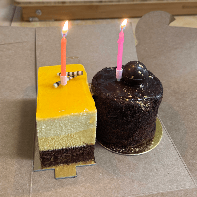
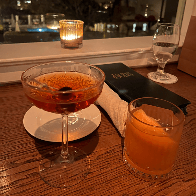
Here are two test images of my own, one with two slices of cakes in it, another taken at a cocktail bar. I denoised these images following the same procedure.

Original

Original

SDEdit with i_start=1

SDEdit with i_start=3

SDEdit with i_start=5

SDEdit with i_start=7

SDEdit with i_start=10

SDEdit with i_start=20

SDEdit with i_start=1

SDEdit with i_start=3

SDEdit with i_start=5

SDEdit with i_start=7

SDEdit with i_start=10

SDEdit with i_start=20

We observe from both test images that the recovery process hallucinates severely until i_start = 20. This shows again that we are essentially just creating images that are similar to the original image, with a low-enough noise level.

1.7.1 Editing Hand-Drawn and Web Images

I then tried using nonrealistic images. Below are two hand-drawn images I created, and we denoised for noise levels [1, 3, 5, 7, 10, 20].

Hand drawn leaf

SDEdit with i_start=1

SDEdit with i_start=3

SDEdit with i_start=5

SDEdit with i_start=7

SDEdit with i_start=10

SDEdit with i_start=20

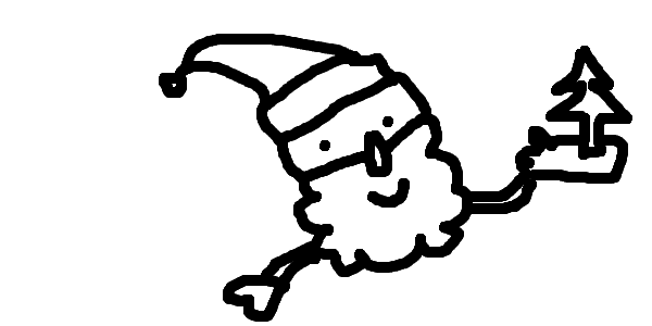
Hand drawn santa

SDEdit with i_start=1

SDEdit with i_start=3

SDEdit with i_start=5

SDEdit with i_start=7

SDEdit with i_start=10

SDEdit with i_start=20

At lower i_start values (SDEdit = [1, 3, 5]), a higher level of noise is added to the input image, which destroys much of the original structure. As a result, the denoising process produces more creative and heavily hallucinated outputs that are often less related to the original hand-drawn images. As the noise level decreases at largeri_start values (e.g., 10 and 20), more structural information is preserved, and the generated images more closely match the style and content of the original hand-drawn inputs.

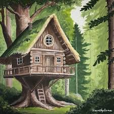
Web image: tree house

I also used an image online to test the procedure out. We observe the same pattern that the less noisy the image is, more similar the denoised image is to the source image.

SDEdit with i_start=1

SDEdit with i_start=3

SDEdit with i_start=5

SDEdit with i_start=7

SDEdit with i_start=10

SDEdit with i_start=20

1.7.2 Inpainting

We can use the same iterative denoise CFG approach to implement inpainting, so we only edit the image part where the mask value is 1. Below is an example of inpainting using the Campanile.

Original

Mask

Hole to Fill

Campanile Inpainted

I then created binary masks for two of my own test images, carving out a chocolate cake and a cocktail glass. During the denoising process, the masked regions are filled in with new content inferred by the model. As a result, the chocolate cake is replaced by a mango cake with icing, and the cocktail glass is replaced with a different glass top, demonstrating how the model can plausibly hallucinate objects within specified masked areas.

Original

Mask

Hole to Fill

Campanile Inpainted

Original

Mask

Hole to Fill

Campanile Inpainted

1.7.3 Text-Conditional Image-to-image Translation

We can also guide the projection of SDEdit with a text prompt. Using the Campanile image and a text prompt A 2D cartoon character, I created image-to-image tranlation at noise level [1, 3, 5, 7, 10, 20].

2D character at noise level 1

2D character at noise level 3

2D character at noise level 5

2D character at noise level 7

2D character at noise level 10

2D character at noise level 20

Using the prompt below, I was able to transform the image of the cocktail bar to an image with a 2D cartoon character in the bar.

prompt = 2D animated, warm and inviting cartoon character in soft pastel colors, flat-vector style. Ethnically neutral, gender-neutral, wearing casual outdoorsy clothes with a backpack. One hand raised in a friendly wave, light gentle smile, relaxed and welcoming posture. Green hoodie, dark blue pants, brown boots, yellow backpack. Eyes looking forward naturally. clean smooth lines, minimal brush strokes, subtle shading, harmonious warm tones, cozy and playful feel, crisp edges, polished and simple, transparent background, full body, centered, game-ready style for animation sprites.

2D character at noise level 1

2D character at noise level 3

2D character at noise level 5

2D character at noise level 7

2D character at noise level 10

2D character at noise level 20

Using the prompt below, I also transformed the image of cakes to an image with a slice of cake and a fancy drone.

prompt = High-detail 3D sci-fi drone rendered in sleek hard-surface style. Metallic cool-tone palette (steel, gunmetal, silver) with subtle emissive blue accents. Compact spherical body with symmetrical quad rotors, glowing energy core at the center. Sharp, precise edges and reflective surfaces. Industrial-futuristic aesthetic inspired by AAA game concept art. Dynamic but stable hover pose. Soft studio lighting, crisp shadows, photorealistic reflections. No background (transparent), clean polished finish, centered, full object, production-ready for robotics concept visualization.

Drone at noise level 1

Drone at noise level 3

Drone at noise level 5

Drone at noise level 7

Drone at noise level 10

Drone at noise level 20

We observe that the original image and the text prompt begin to visually merge at higher noise levels (around i_start = 10 and 20), because at lower noise levels the masked SDEdit images retain too much of the original structure, limiting the model’s ability to integrate the new prompt.

1.8 Visual Anagrams

I created two paris of visual anagrams with diffuson models. To do this, we will denoise an image $x_t$ at step $t$ normally with the prompt $p_1$, to obtain noise estimate $\epsilon_1$. But at the same time, we will flip $x_t$ upside down, and denoise with the prompt$p_2$, to get noise estimate $\epsilon_2$. We can flip $\epsilon_2$back, and average the two noise estimates. We can then perform a reverse diffusion step with the averaged noise estimate.

I started with the example prompt pairs, and created a flipped visual anagram pair of an old man and people around a camp fire.

An Oil Painting of an Old Man

An Oil Painting of People around a Campfire

I also created another pair with a queen and a christmas tree.

A portrait of a queen

A painting of a christmas tree

1.9 Hybrid Images

We can create ahybrid images by creating a composite noise estimate, with two different text prompts. We combine low frequencies from one noise estimate with high frequencies of the other. It achives similar effects as hybrid images from Project 2, where the zoomed in and out versions of the images are different.

Below are the two hybrid images I created, by combinig a house plant with the Statue of Liberty, and a polar bear with a dining table.

Close up: a watercolor painting of a house plant

Far away: a watercolor painting of the statue of liberty

Hybrid image of a house plant and the statue of liberty

Close up: a oil painting of a dining table

Far away: an oil painting of a polar bear

Hybrid image of a polar bear and a dining table

More visual anagrams!

We can also create more transformations for visual anagrams than just flipping it upside down.

Negative anagram

Compared to the flipped visual illusion, negative visual anagrams work by performing pixel-wise negation of the image. To compute the composite noise, I get the noise for the bright image and the dark image, as the dark image is just negativing every pixel in the bright image. Then I sum the absolute value of both noise to get the composite noise estimate. I then follow the same steps as the flipped image generation process, to get the final visual results.

a lithograph of a teddy bear

a lithograph of a rabbit

Skewed anagram

To create skewed visual anagrams, we follow the same process as the other visual anagrams. We also invert the permuted (skewed) view’s noise before averaging it with the original view. I manipulated the image by applying column-wise shifts, to roll parts of the image horizontally. This creates a rearranged structure within the image.

a watercolor painting of the statue of liberty

a watercolor painting of a house plant

Design a course logo!

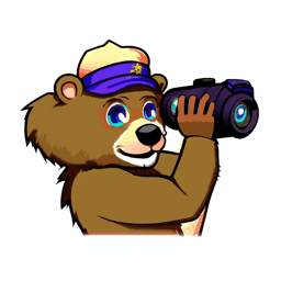
To design a course logo, I used text-conditioned image-to-image translation. I started with an image of Oski, and conditioned with the prompt below.

Oski

SDEdit with i_start=1

SDEdit with i_start=3

SDEdit with i_start=5

SDEdit with i_start=7

SDEdit with i_start=10

SDEdit with i_start=20

Prompt: a 2D animated University of California at Berkeley's bear Oski holding a camera

Then, I picked the best visual effect at i_start = 10, and upscaled the image to get the course logo.

Best course logo (SDEdit = 10)

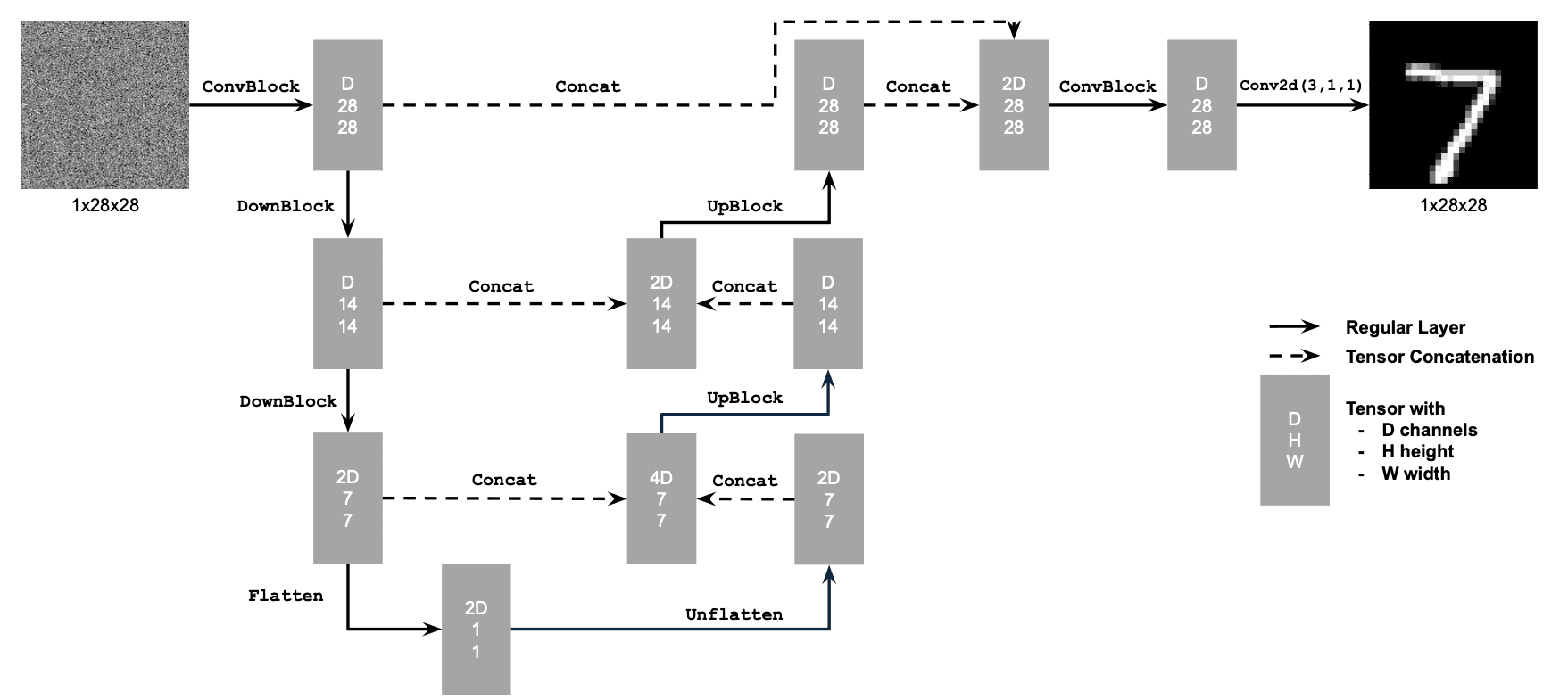
1.1 Implementing the UNet

The first step in this project is to build a simple one-step denoiser. Given a noisy image $z$, we aim to train a denoiser $D_{\theta}$ such that it maps $z$ to a clean image $x$. To do so, we can optimize over an L2 loss:

To build the denoiser, I followed the architecture below:

1.2 Using the UNet to Train a Denoiser

To train our denoiser, we need to generate training data pairs of $(z, x)$, where each $x$ is a clean MNIST digit. For each training batch, we can generate $z$ from$x$ using the the following noising process:

Below is a visualization of the noising process, using $\sigma = [0.0, 0.2, 0.4, 0.5, 0.6, 0.8, 1.0]$

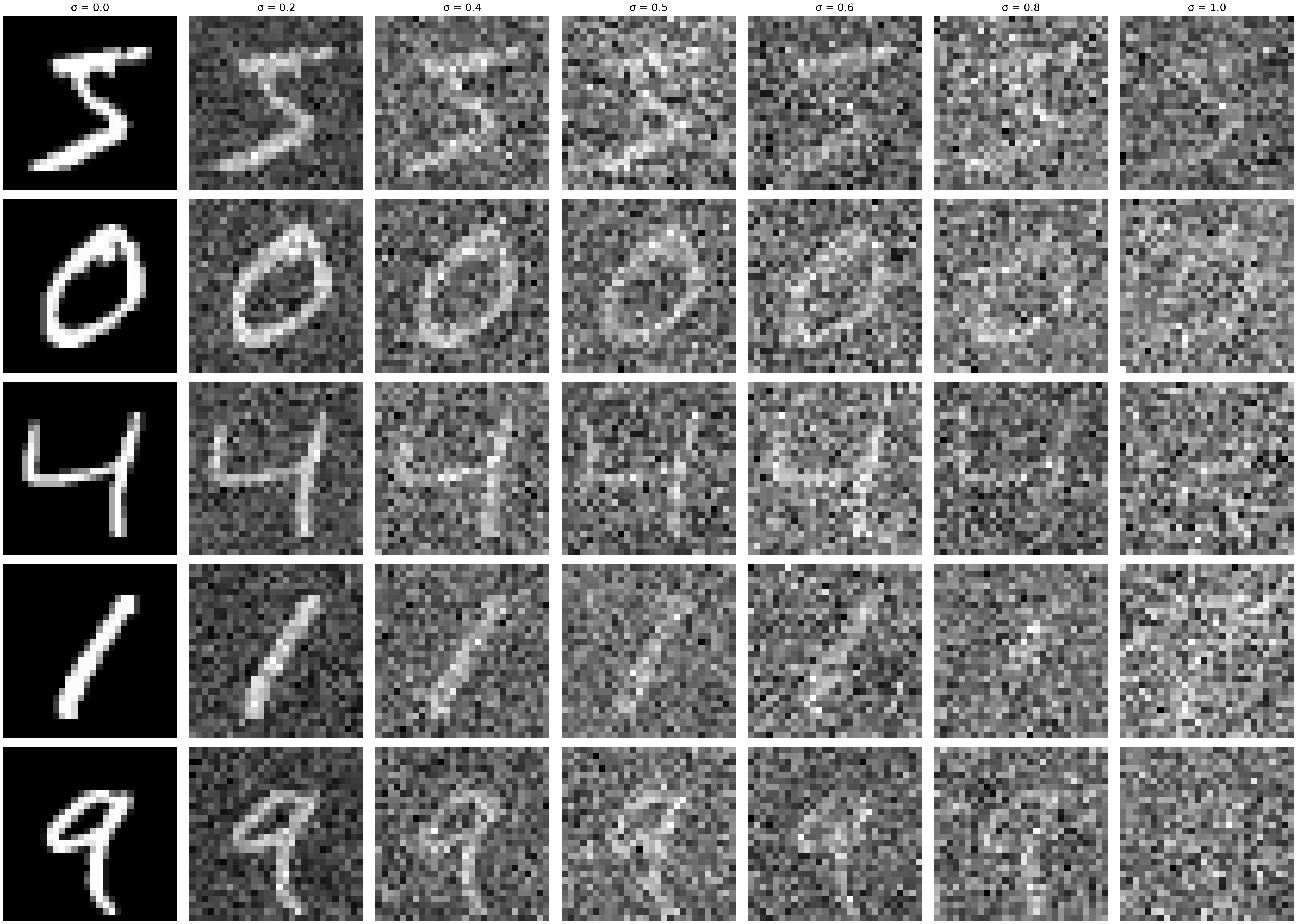
As we see above, the noisy image $z$ gets more noisy as we increase the sigma value. When $\sigma = 1.0$, we get a completely blurry image with all pixels randomly generated from a normal distribution with mean 0 and variance 1.

1.2.1 Training

Now, we will train the model to perform denoising on noisy image $z$ with $\sigma = 0.5$ applied to a clean image $x$.

In this section, I am using the UNet architecture defined in section 1.1, with an Adam optimizer. Here are the hyperparameters I used for this training task:

batch_size = 256
learning_rate = 1e-4
noise_level = 0.5
hidden_dim = 128
num_epochs = 5

To imporve generalization, I only noise the image batches when fetched from the dataloader so that in every epoch the network will see new noised images due to a random $\epsilon$.

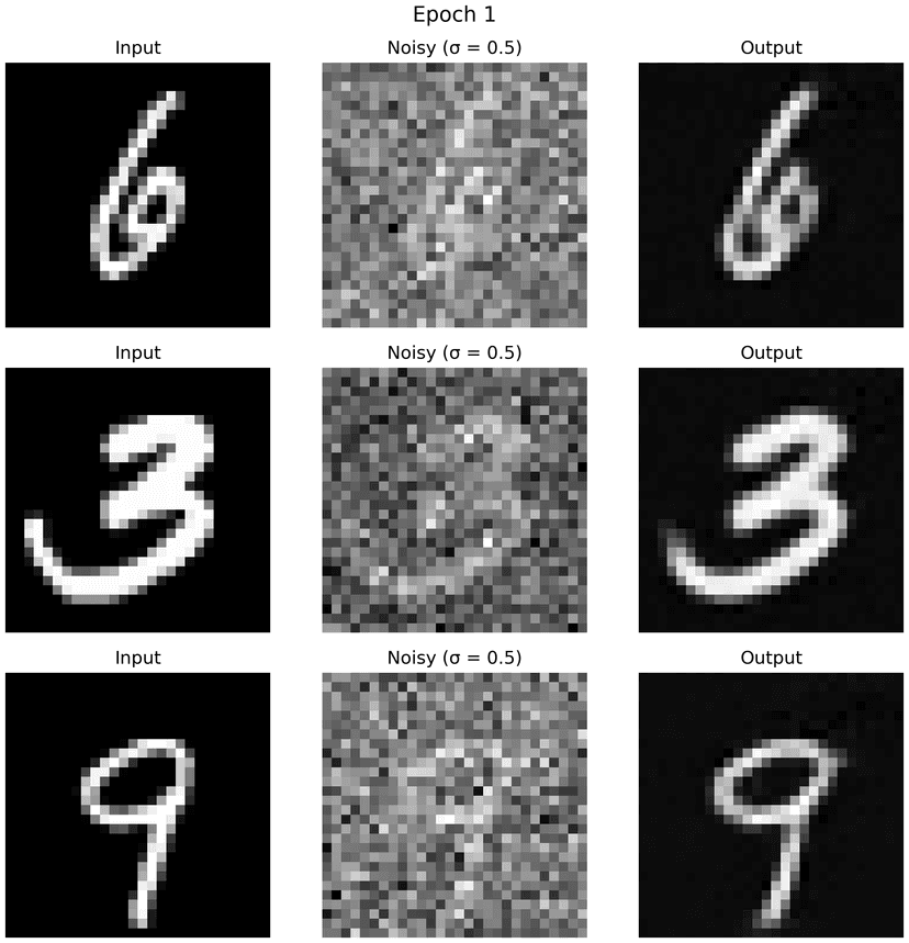
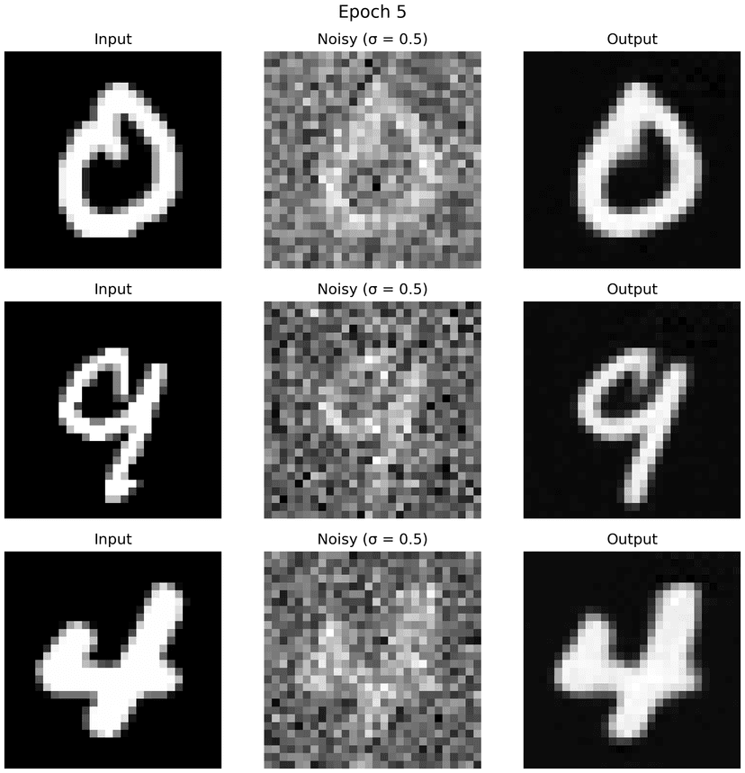
Below are the results on the test set, with noise level 0.5, after the first and the 5-th epoch.

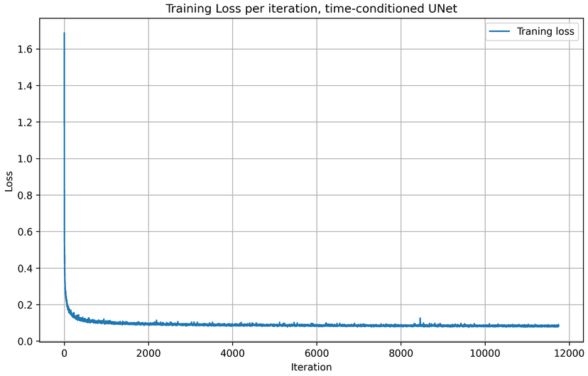
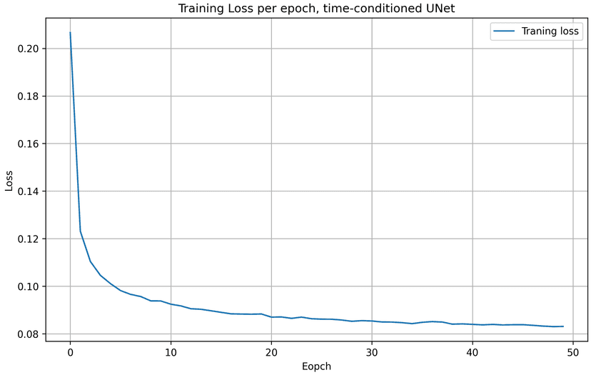
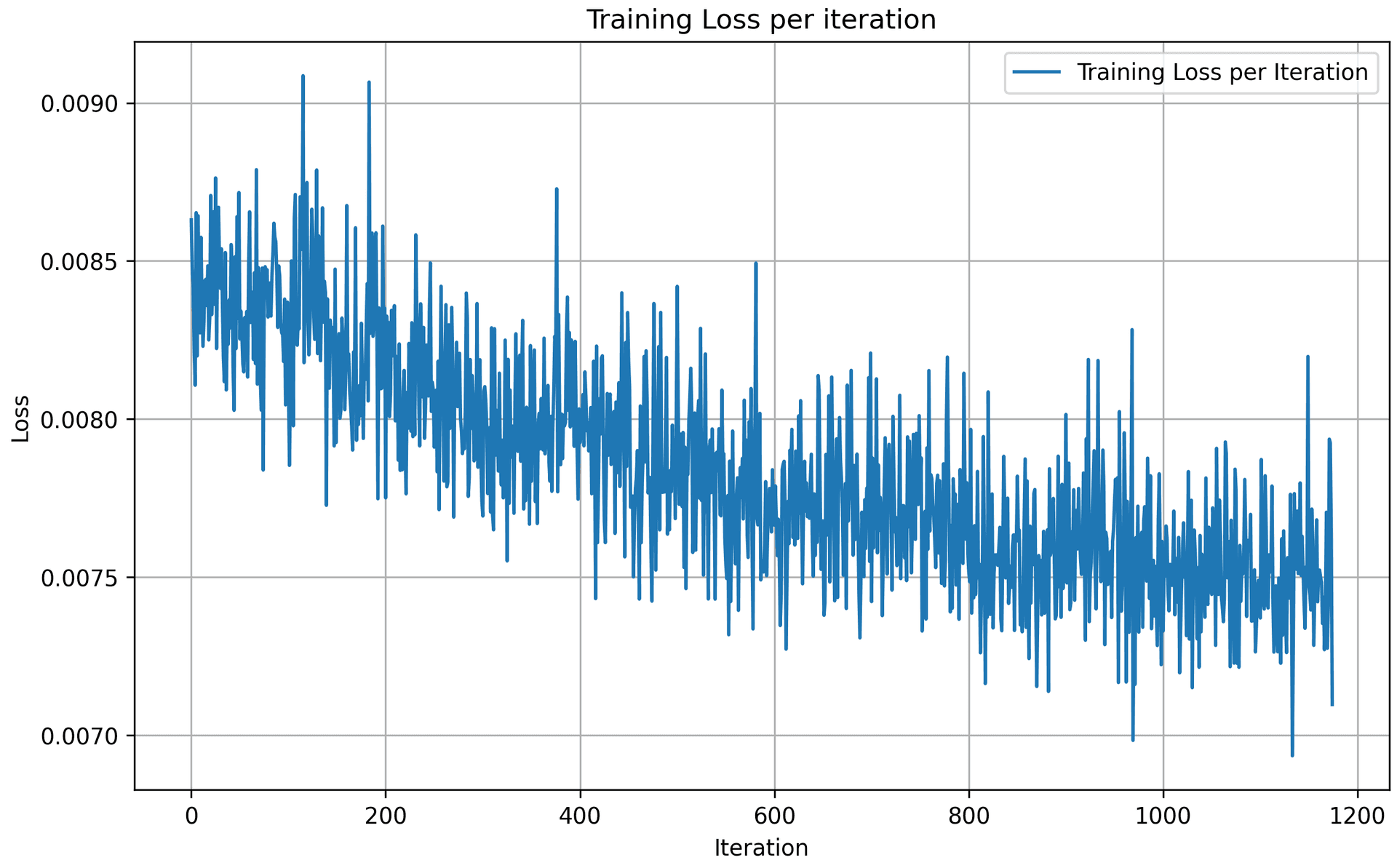
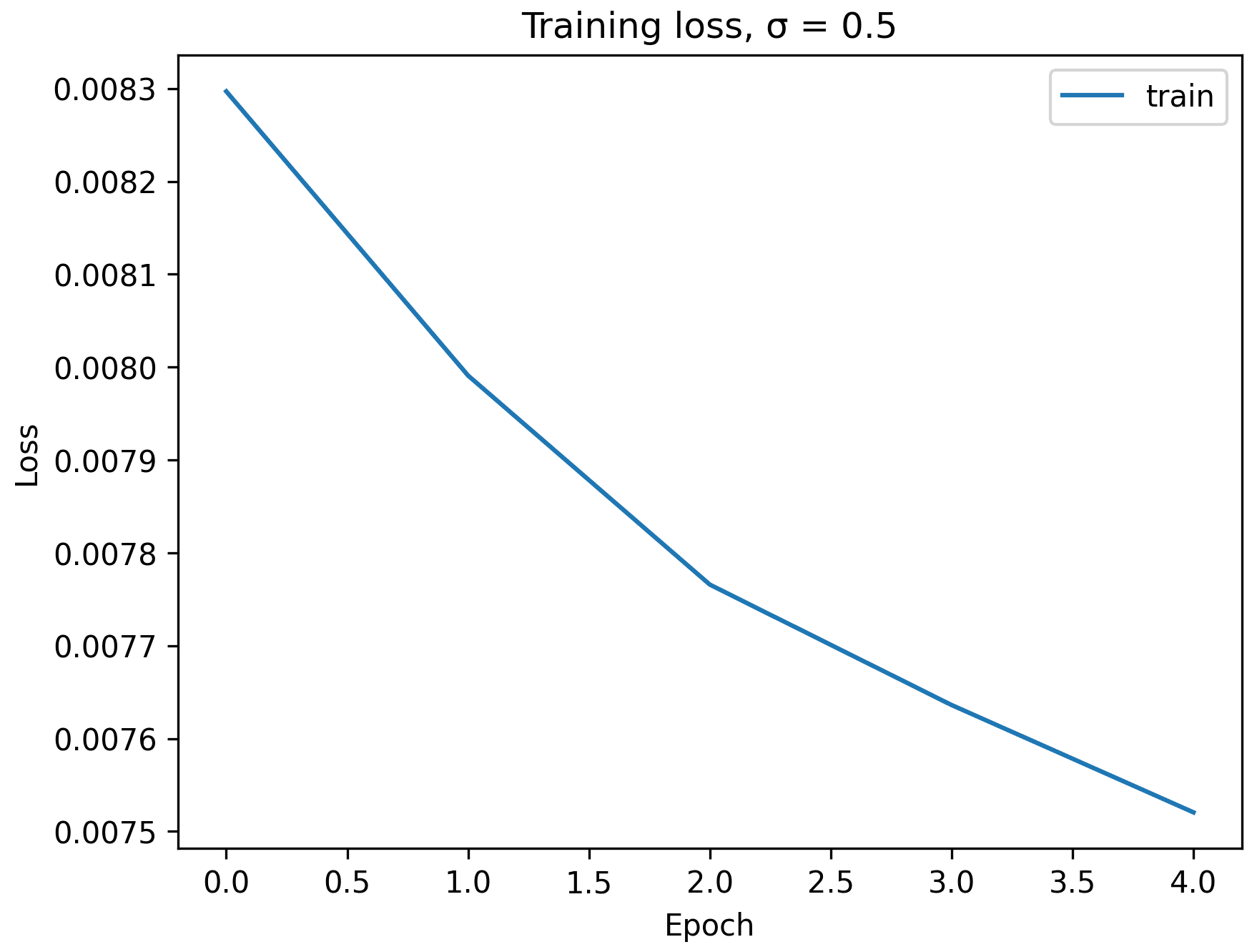
Here are the training loss curve plots for every iterations and epochs during the whole training process, with noise level = 0.5. Due to the scale, the training loss per iteration is not a smooth curve going down, but the training loss per epoch shows that the model indeed converges and loss reduces over eopchs.

1.2.2 Out-of-Distribution Testing

The above denoiser is trained on $\sigma = 0.5$. To see how the denoiser performs on different noise levels, we apply the denoiser on images with various noise levels, $\sigma = [0.0, 0.2, 0.4, 0.5, 0.6, 0.8, 1.0]$

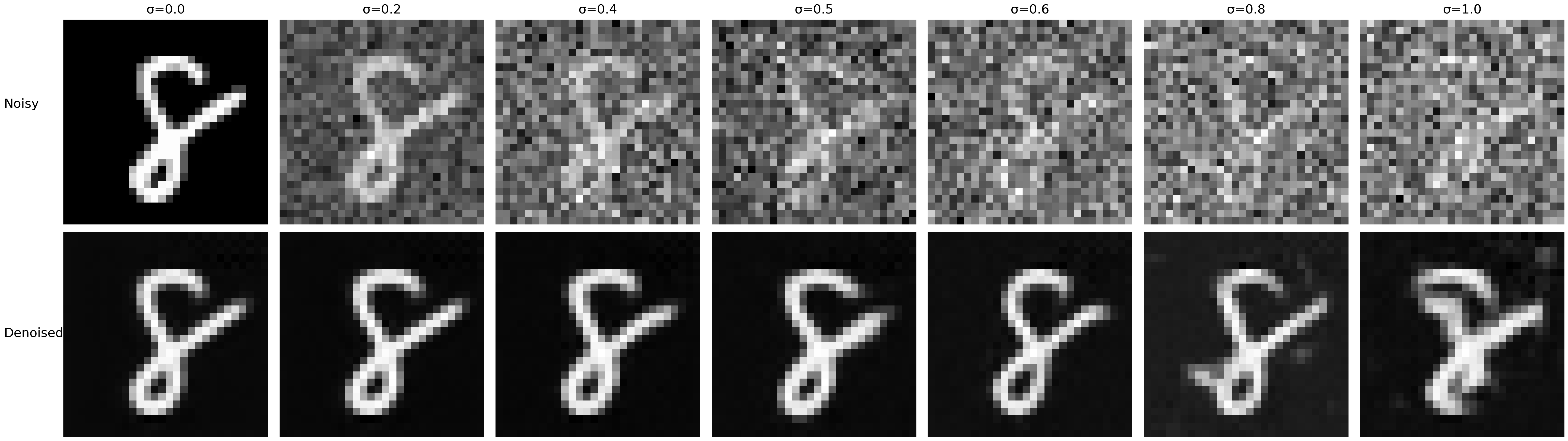
We see that the denoiser works generally pretty well for lower noise levels, $\sigma = [0.0, 0.2, 0.4, 0.5, 0.6]$, while the denoised images for $\sigma = [0.8, 1.0]$ get blurry with redundant white pixels outside of the digit figure. These additional noise were not removed during the denoising process, because the denoiser was only trained on noise level = 0.5.

1.2.3 Denoising Pure Noise

To make denoising a generative task, we would like to be able to denoise pure, random Gaussian noise. To get the noisy image, instead of starting with a clean image $x$ to get the noisy image $z$, we would need to start from a blank canvas and apply noise to it. So we have $z = \epsilon$ where $\epsilon \sim N(0, I)$.

Now, we repeat the training process in part 1.2.1 for 5 epochs. Below are the results on pure noise after the first and the 5-th epoch.

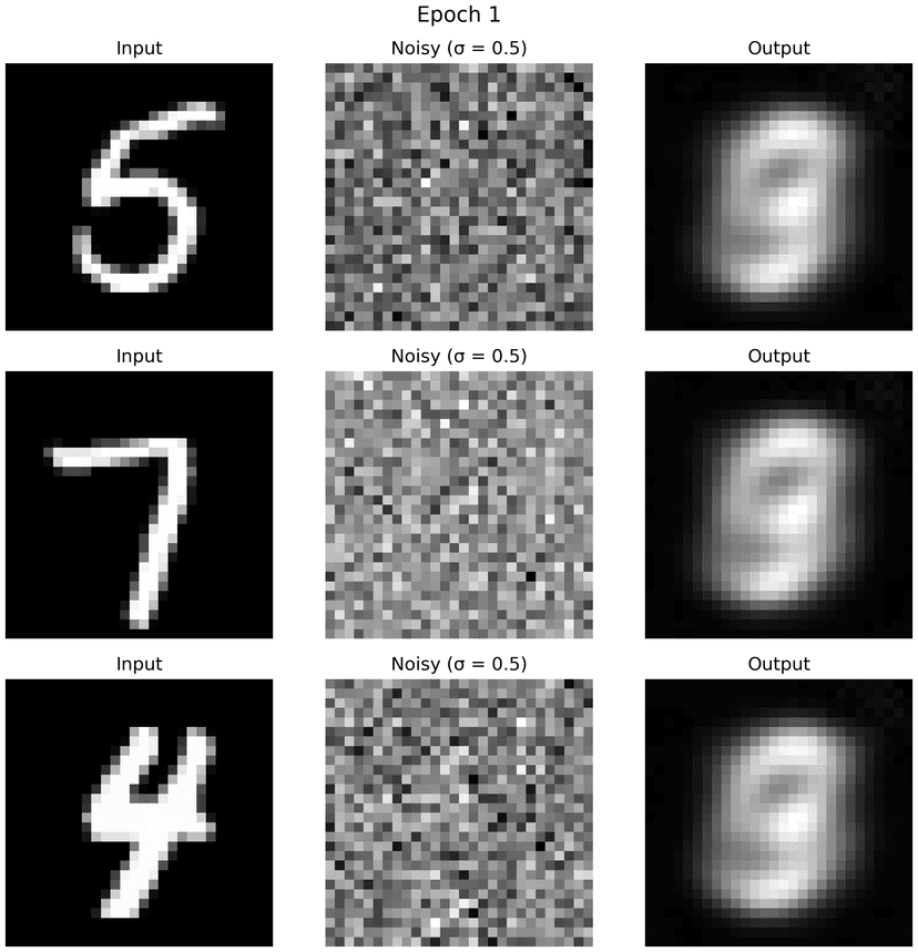
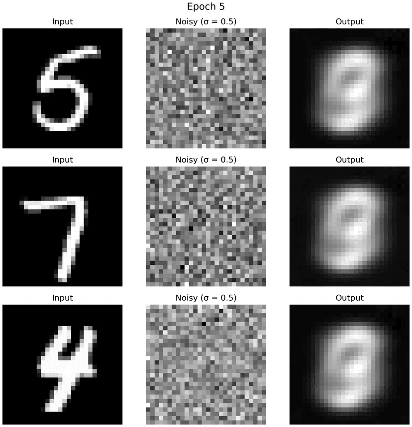
We see that the generated outputs above appear as blurry and ambiguous figures that resemble digits but are not clearly recognizable as any specific number. This is because, unlike the standard denoising setting where the noisy input $z = x + \epsilon$ contains an underlying clean image $x$, pure noise $z = \epsilon$ does not contain any recoverable signal. As a result, the denoising task becomes ill-posed: there is no unique clean image that the model should reconstruct from the input.

Under an MSE-based objective, the denoiser learns to predict the conditional expectation of the clean image given the noisy input. When the input is pure noise, this conditional distribution is highly uncertain and spans many possible digits. Consequently, the model produces outputs that resemble an average over the training data distribution, leading to smooth, low-frequency, and blurry digit-like shapes rather than sharp, class-specific structures.

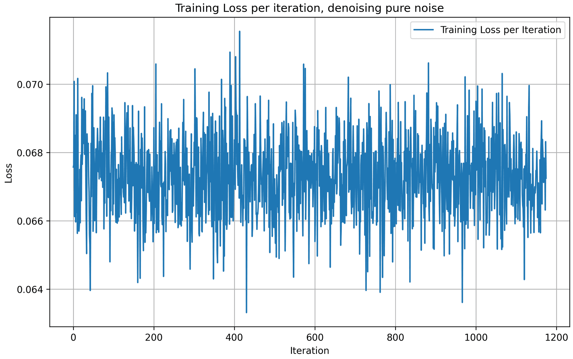
We also observe that the training loss over iterations does not consistently decrease. This is because pure noise inputs do not correspond to a stable or well-defined target output, making it difficult for the model to learn a consistent input–output mapping. Without an underlying clean image to guide reconstruction, gradient updates become noisy and the optimization process lacks a clear direction for convergence.

These results above highlight that denoising pure noise alone is insufficient to produce a meaningful generative model. We need a strong input signal on what the image represents, rather than just a normal distribution of noise, to yield convergence and results.

Part 2: Training a Flow Matching Model

We just saw that one-step denoising does not work well for generative tasks. Instead, we need to iteratively denoise the image, and we will do so with flow matching. Here, we will iteratively denoise an image by training a UNet model to predict the flow from our noisy data to clean data.

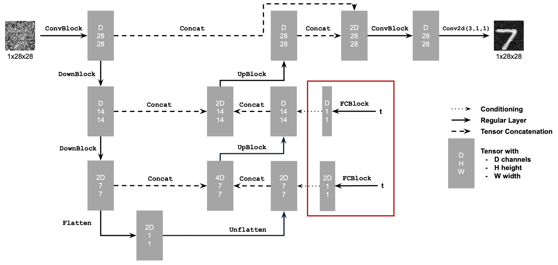
2.1 Adding Time Conditioning to UNet

I followed the architecture below to enhance the above UNet model, by injecting scalar t into it to condition it.

2.2 Training the UNet

Now, we will train this time-conditioned UNet model $u_{\theta}(x_{t}, t)$ to predict the flow at $x_t$ given a noisy image $x_t$and a timestep $t$.

In this section, I am using the time-conditioned UNet architecture defined in section 2.1, with an Adam optimizer and an exponential learning rate decay scheduler. Here are the hyperparameters I used for this training task:

batch_size = 256
learning_rate = 1e-2
noise_level = 0.5
hidden_dim = 64
num_epochs = 10

gamma = 0.1 ** (1.0 / num_epochs)
scheduler = torch.optim.lr_scheduler.ExponentialLR(optimizer, gamma=gamma)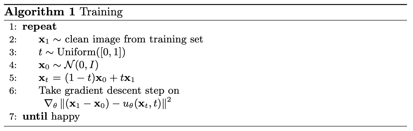

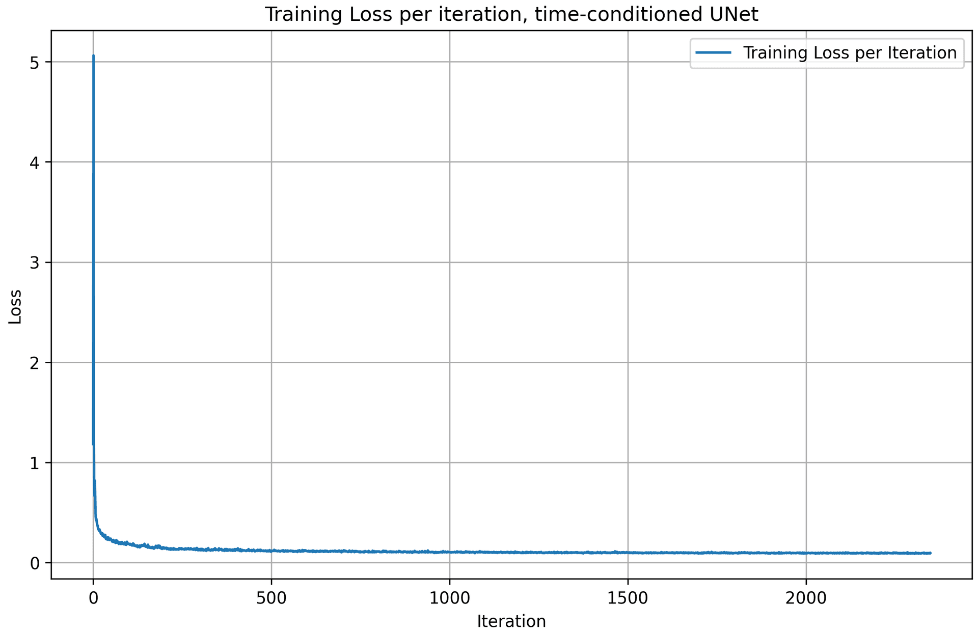
Following the algorithm above, we get a training loss curve plot for the time-conditioned UNet over the whole training process. The model quickly converges after a few iterations, as the loss value drops very fast.

2.3 Sampling from the UNet

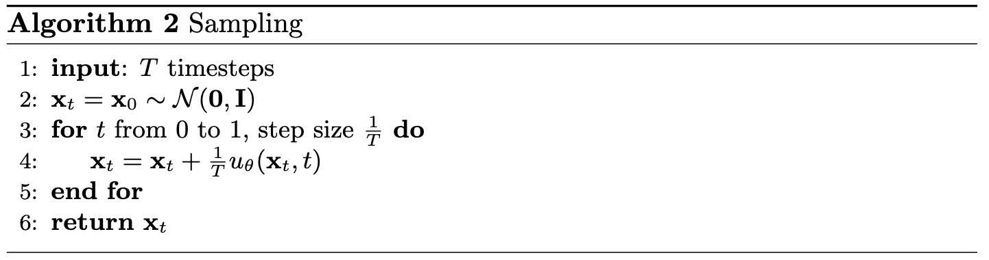
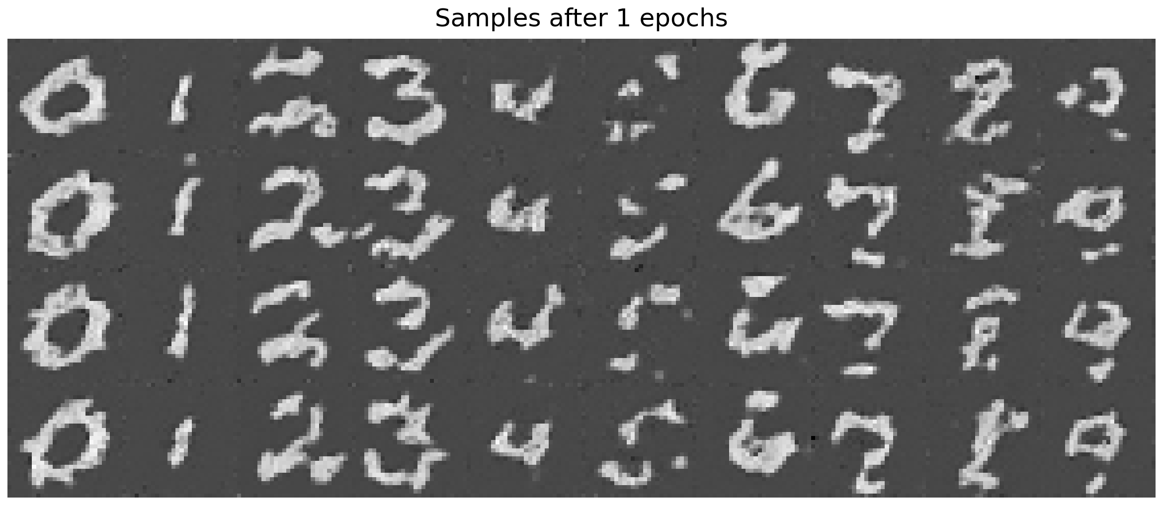
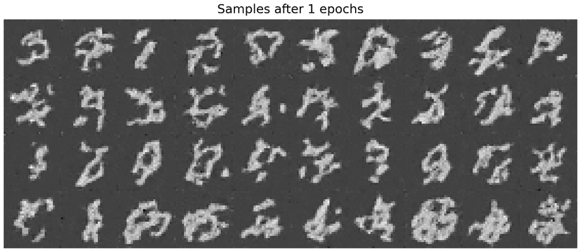
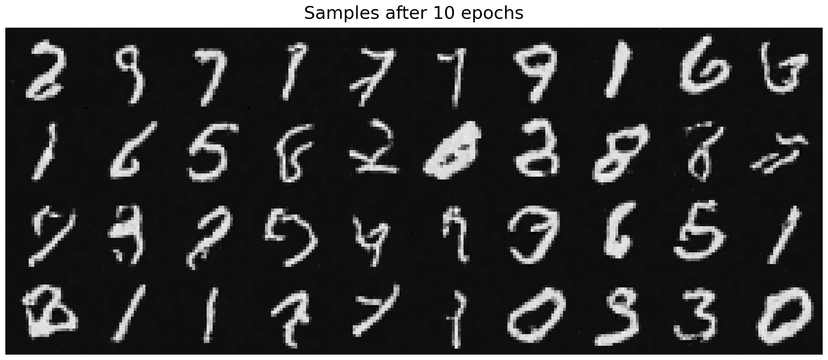
Following the sampling algorithm described above, we generate samples from the time-conditioned UNet after 1, 5, and 10 epochs of training, with 40 images sampled at each epoch. As training progresses, the quality of the generated samples improves noticeably. In particular, samples from later epochs exhibit clearer digit-like structures compared to those from earlier epochs.

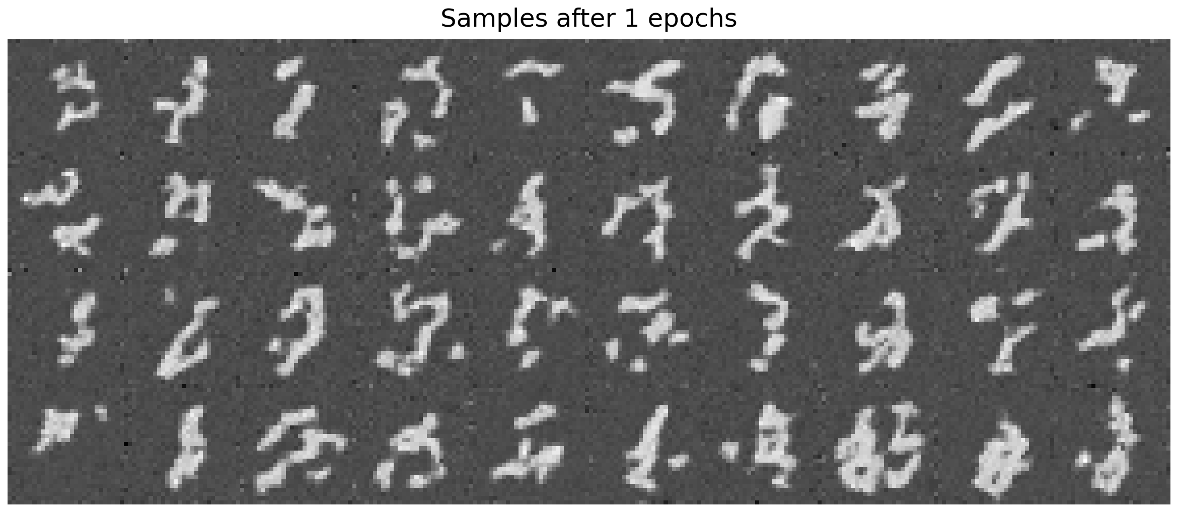
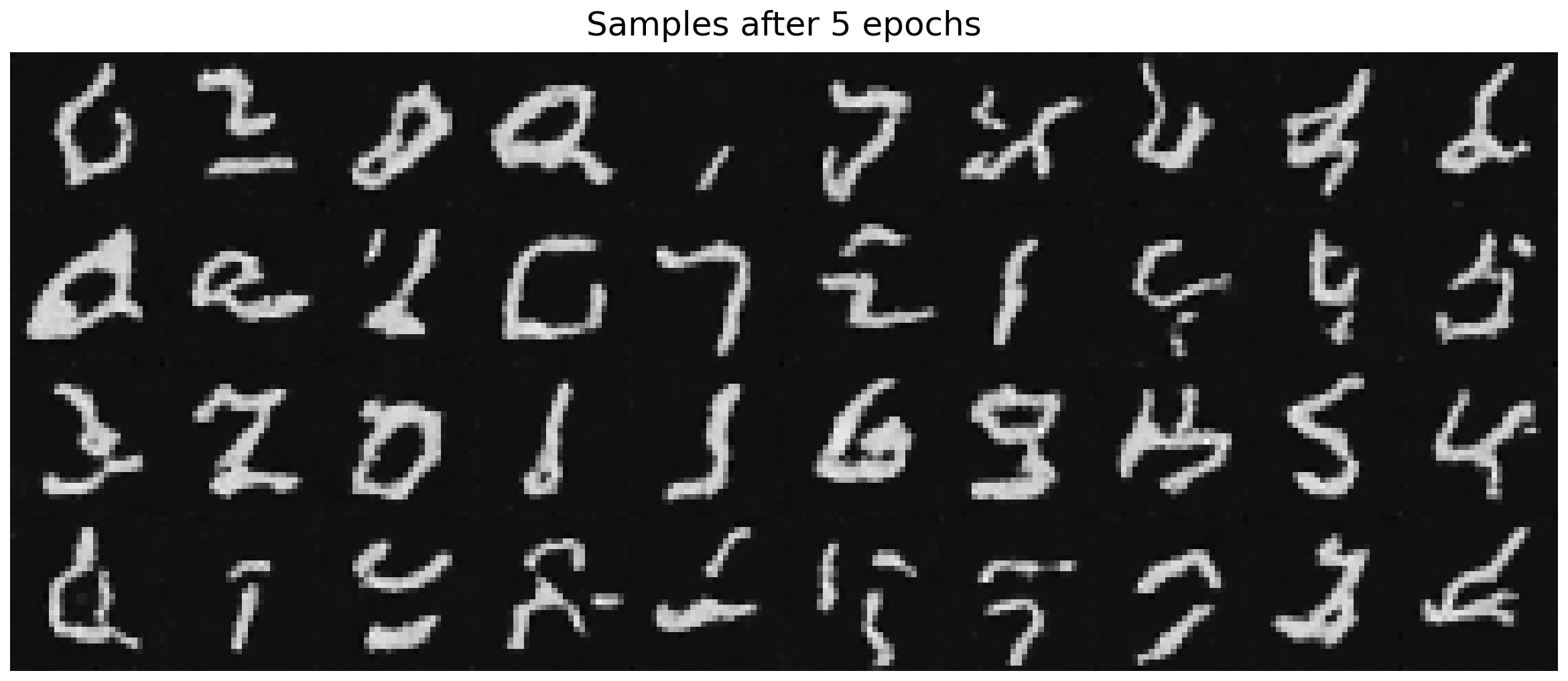
However, even at epoch = 10, the generated digits remain imperfect. While some digits are partially recognizable, many samples appear blurry or resemble scribbles rather than well-defined numbers. This suggests that time-only conditioning provides the model with insufficient guidance to fully capture the underlying data distribution. Without additional conditioning signals such as class labels or a more expressive architecture, the model struggles to generate sharp, semantically consistent digit shapes.

2.4 Adding Class-Conditioning to UNet

To make the results better and give us more control for image generation, we can also optionally condition our UNet on the class of the digit 0-9. I added 2 more FCBlocks to the UNet, as well as a one-hot vector $c$ for class-conditioning. Because we still want our UNet to work without it being conditioned on the class, I implemented dropout where 10% of the time ($p_{\text{uncond}} =0.1$) I drop the class conditioning vector by setting it to 0.

2.5 Training the UNet

Using the same hyperparameters as part 2.2, I trained the time-and-class-conditioning UNet with 5 epochs.

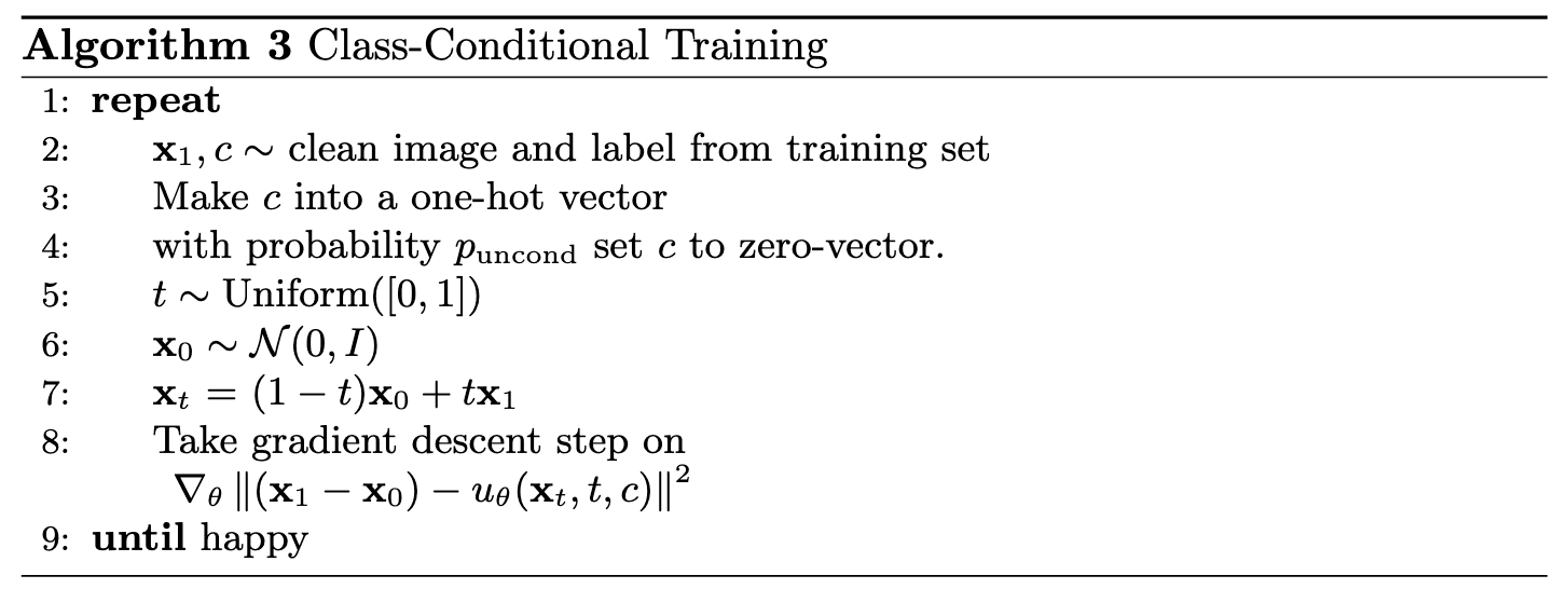
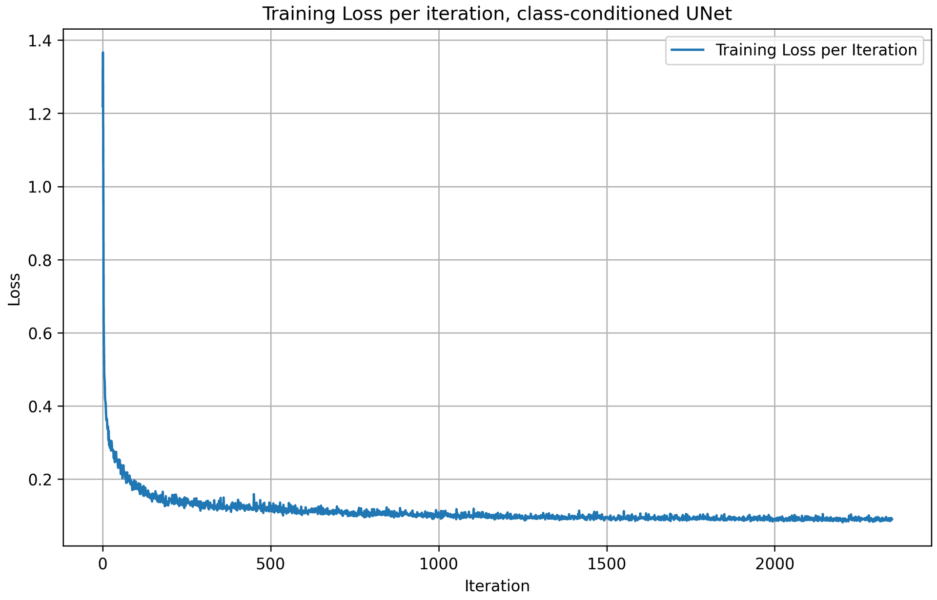
Following the algorithm above, we get the training loss curve plot for the class-conditioned UNet over the whole training process. The model quickly converges after a few iterations, as the loss value drops quickly.

2.6 Sampling from the UNet

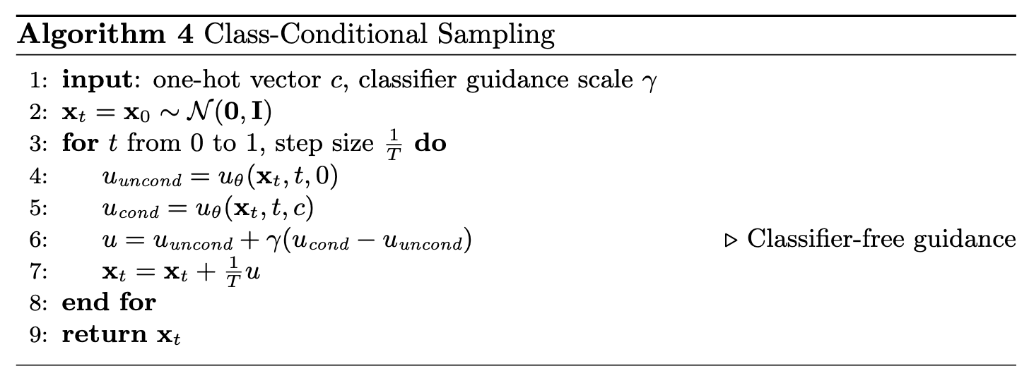
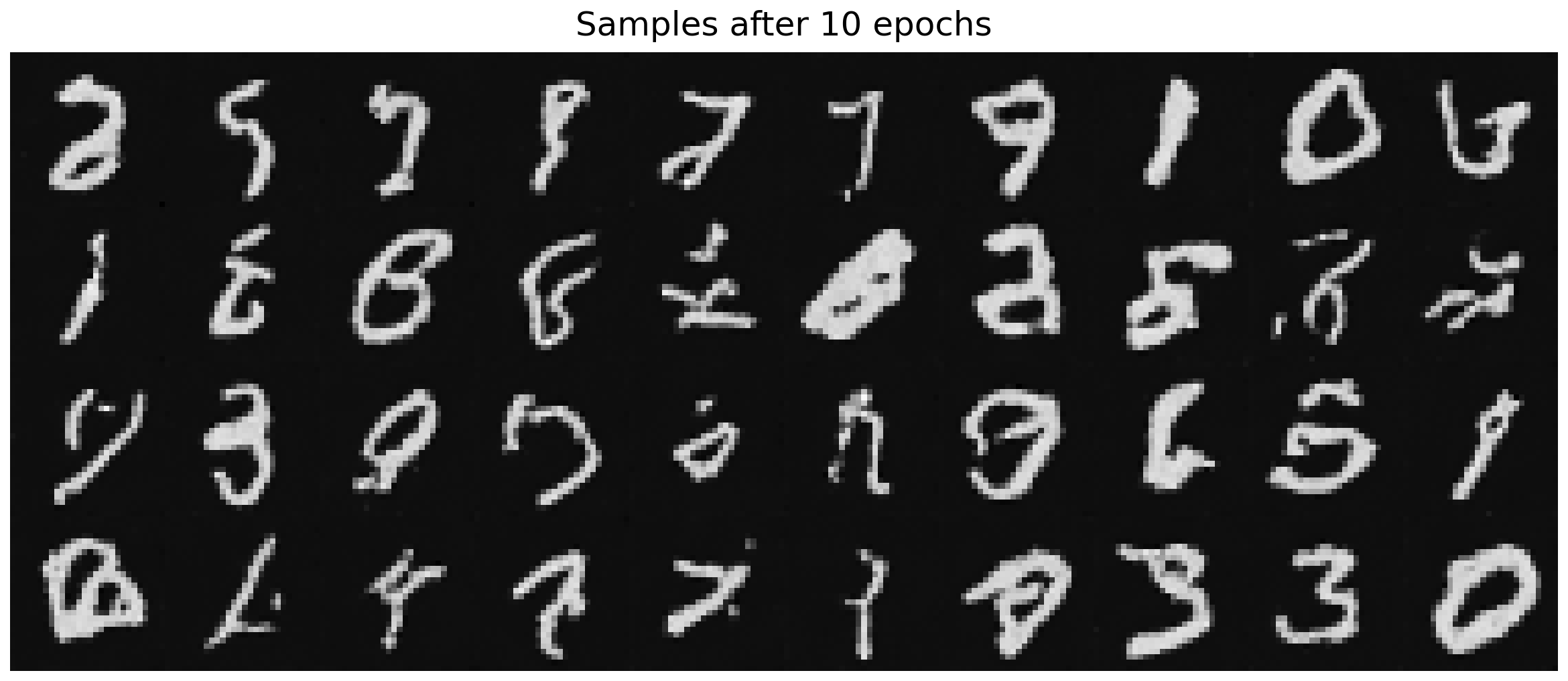
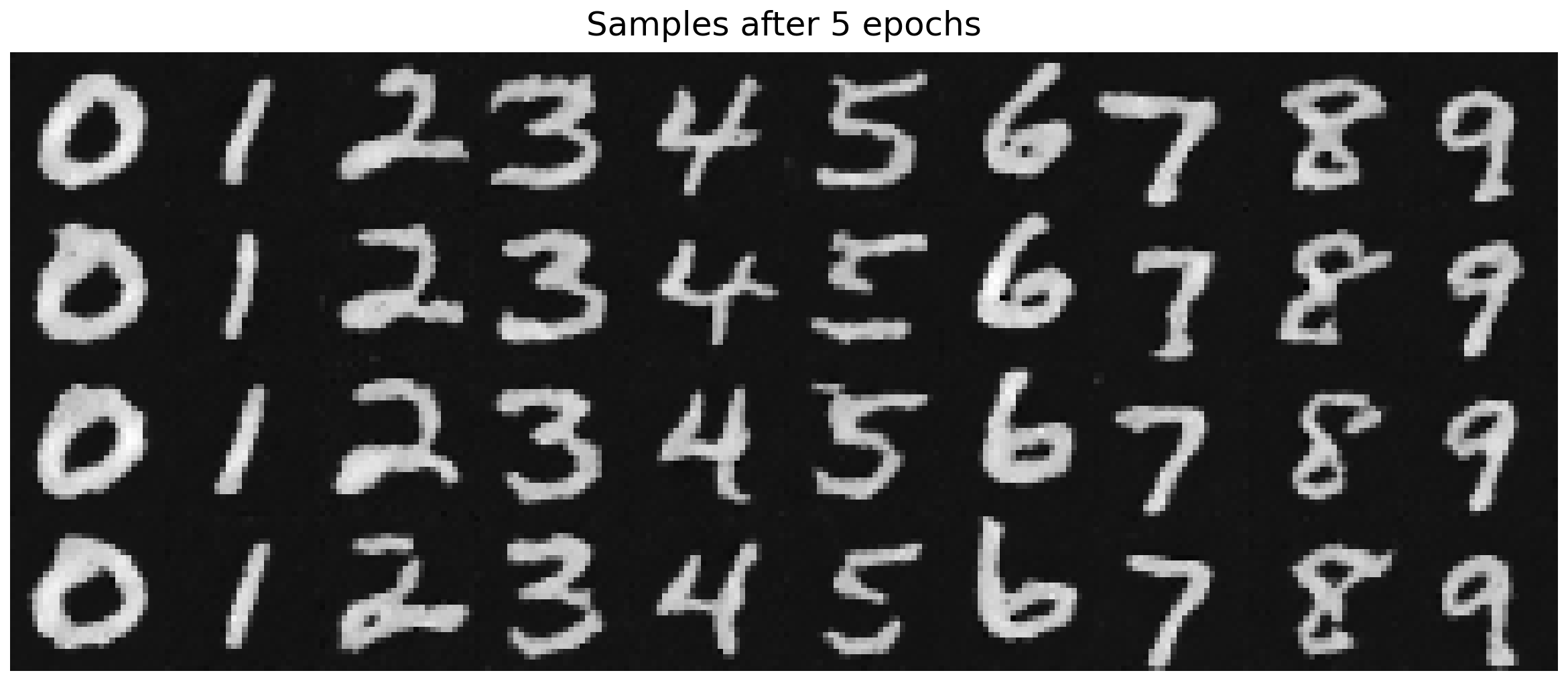
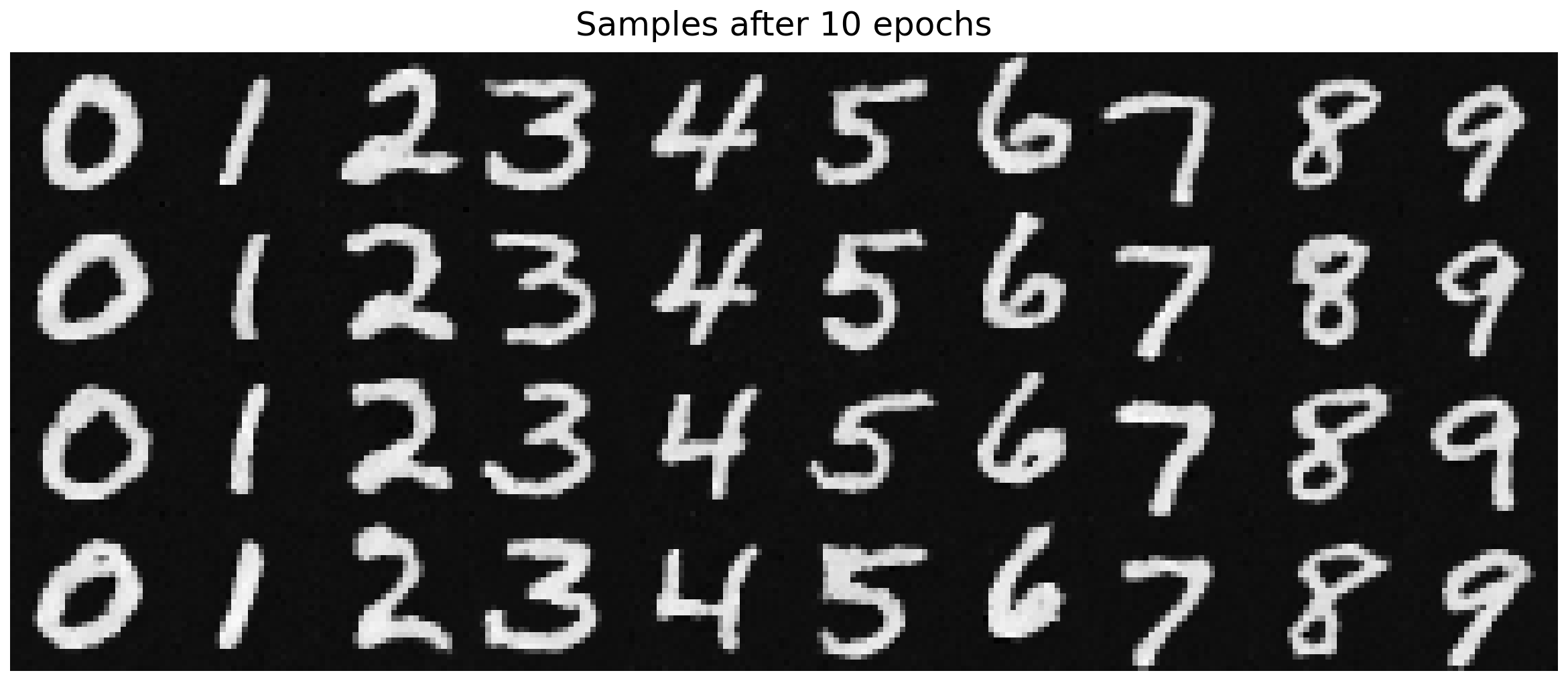
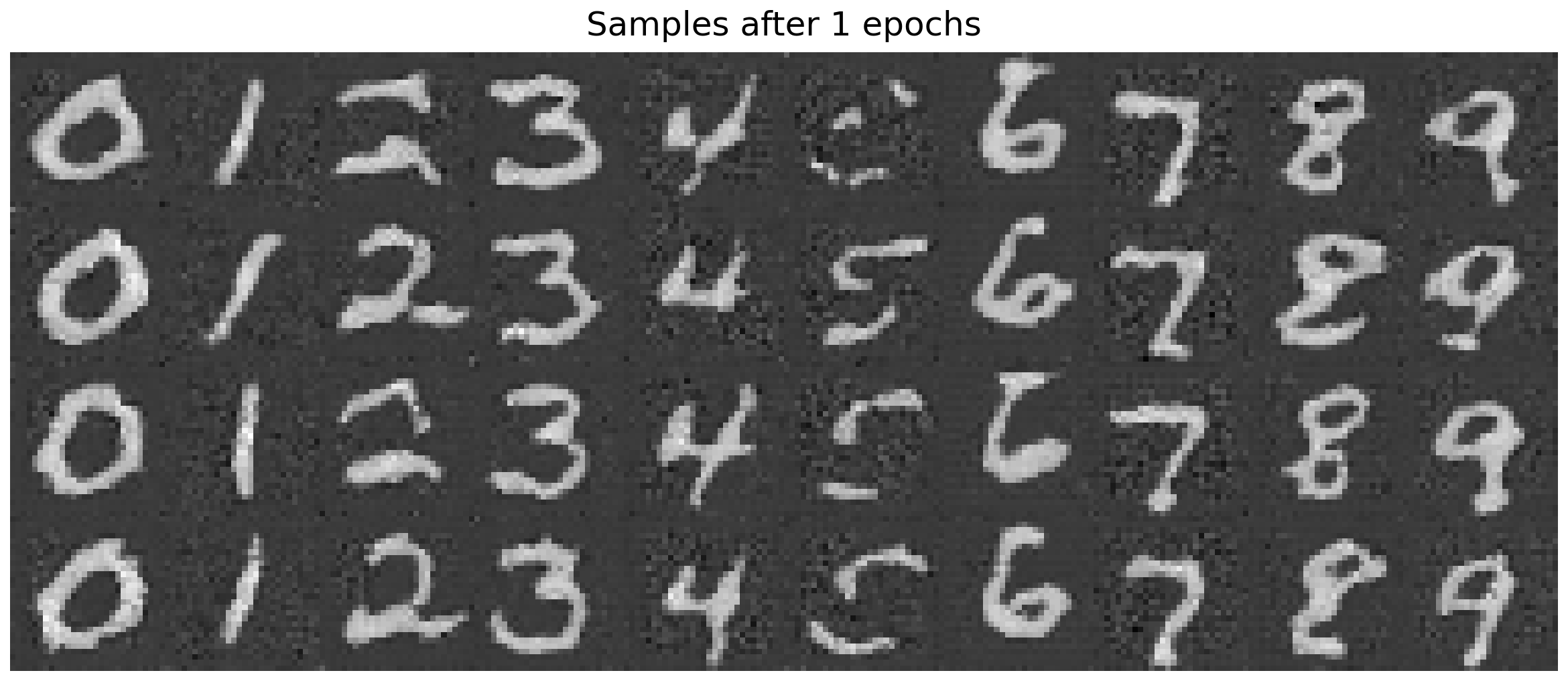
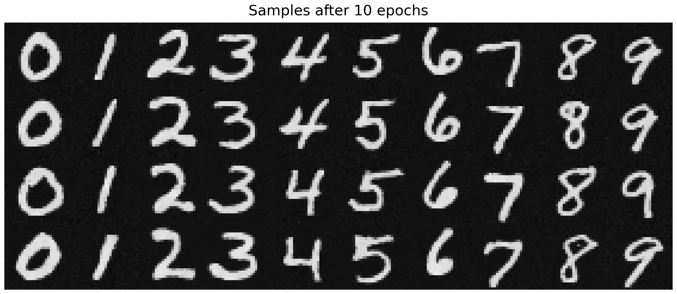
Following the sampling algorithm described above, we generate samples from the class-conditioned UNet after 1, 5, and 10 epochs of training, with 40 images sampled at each epoch. As training progresses, the quality of the generated samples improves noticeably. Even when epoch = 5, the quality of the sampling results is already really good, with clear, recognizable digits in display.

2.6.1 Getting rid of learning rate scheduler

The exponential learning rate scheduler was doing only one thing: gradually reduce the effective step size to stabilize late training. To remove it while achieving similar performance, If we remove it, we must replace that stabilizing effect in some other way.

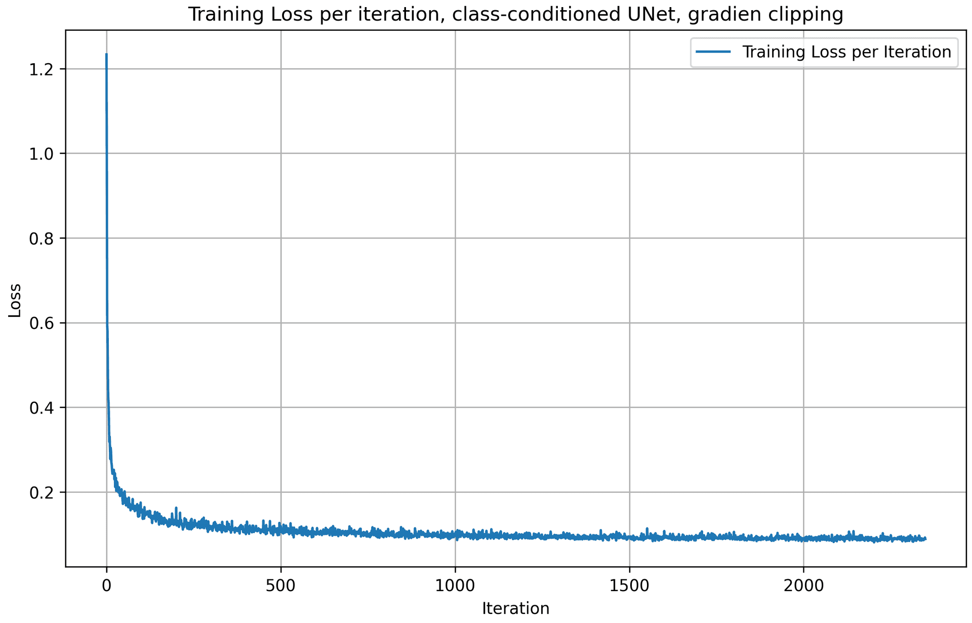
I decided to use gradient clipping here to replace the exponential learning rate scheduler. While exponential decay reduces the step size over time, gradient clipping reduces the magnitude of parameter updates per step. Both aim to keep the updates stable.

With gradient clipping, I set the learning rate to be 1e-3, slightly smaller than the original 1e-2 when using exponential learning rate scheduler. Below is the training loss curve plot for the class-conditioned UNet + gradient clipping, over the whole training process.

batch_size = 256
learning_rate = 1e-3
noise_level = 0.5
hidden_dim = 64
num_epochs = 50

Here are the results from the gradient clipping method, for 1, 5, and 10 epochs. The quality of the results are pretty good and stable for epoch 5 and 10, similar to the above approach with exponential LR scheduler.

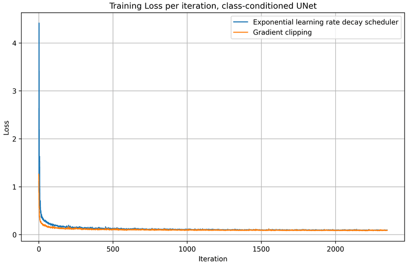
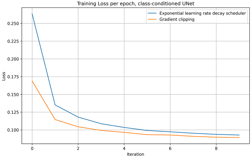
To compare the exponential LR scheduler method with the gradient clipping approach in this section, I compared the iteration and epoch traning loss of both methods and plotted them in the charts below. With a static, slightly smaller learning rate and gradient clipping, we achive slightly better results over 10 epochs of training, comparing to the scheduler approach.

A better time-conditioned only UNet

The time-conditioning only UNet in part 2.3 is actually far from perfect. Its result is way worse than the UNet conditioned by both time and class. To make the time-conditioning only UNet better, an naive approach I took was to increase the training epochs from 10 to 50.

batch_size = 256
learning_rate = 1e-2
noise_level = 0.5
hidden_dim = 64
num_epochs = 50

gamma = 0.1 ** (1.0 / num_epochs)
scheduler = torch.optim.lr_scheduler.ExponentialLR(optimizer, gamma=gamma)

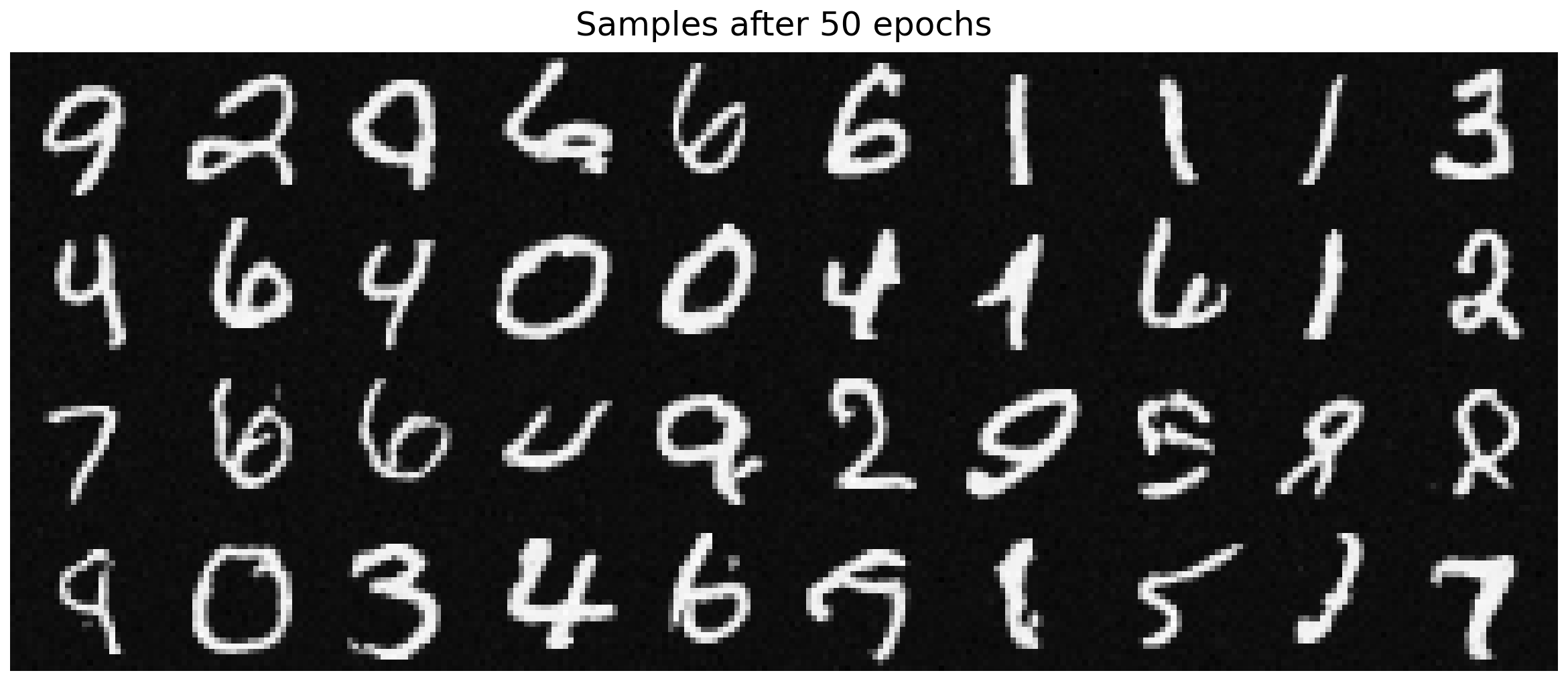
Below are the sample results visualized from every 10 epochs:

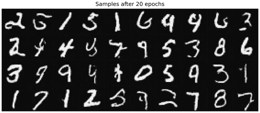
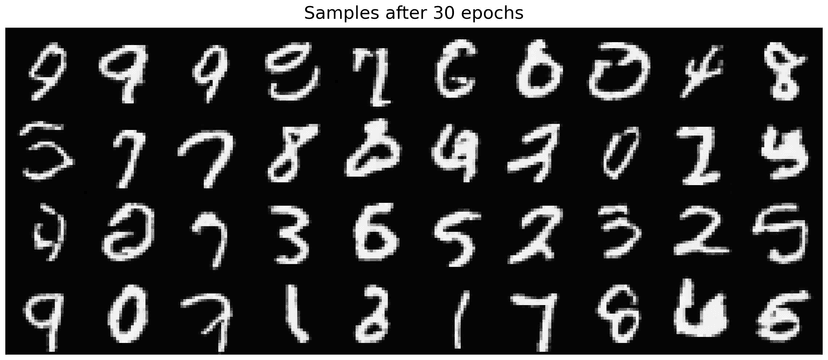
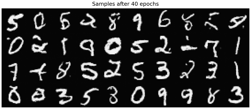
As shown in the visualization, samples generated at the final epoch (epoch = 50) are noticeably clearer and of higher quality compared to those generated at epoch = 10. In particular, the number of scribble-like artifacts is reduced, and the digit structures become more distinct and recognizable. This indicates that extending the training schedule allows the time-conditioned UNet to better learn the denoising dynamics over time.

Here are the training loss curves for training epoch = 50. Comparing to the loss curves for training epoch = 10, we see that the time-conditioning UNet model yields to lower loss values with a larger training epoch.